2.sem

title : ‘[PLS-SEM] 2. Structural Equation Modelling’ categories : ‘SEM’ tag : [‘stat’, ‘PLS’, ‘PLS-SEM’] toc : true date : 2022-08-25 last_modified_at : 2022-08-25

• 본 게시글의 내용은 다음 논문을 참고했습니다.
• semPLS : Structural Equation Modeling Using Partial Least Squares

1. PLS path models

• 3 Components
  1. Structural model
  2. Measurement model
  3. Weighting scheme

• Structural model(구조모델)과 measurement model(측정모델)은 모든 구조방정식 모델(CB-SEM)에 존재하지만 Weighting scheme은 PSL-SEM에만 존재한다.

• PLS-SEM에서 하나의 manifest variable은 하나의 latent variable에만 연결된다. 또한, 하나의 방향만을 가진다. (vs CB-SEM은 순환모델이 가능.) 이때, manifest variable과 latent variable의 연결은 measurement model 또는 outer model이라고 불린다.

  
  

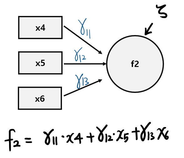
• 방향성이 outer 방향을 향하는 모델을 reflective model(반영모델)이라고 하며, inner 방향을 향하는 모델은 formative model(형성모델)이라고 한다.

반영모델	형성모델

2. Three components

2.1. The structural model

$Y$를 latent variable의 벡터, $B$ 를 계수의 벡터, $Z$를 $E[Z]=0$ 을 만족하는 오차항이라고 할 때,
\(Y = YB + Z\)
가 성립한다.

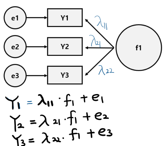
2.2. The measturement model

• 하나의 MV는 하나의 LV에 연결되어야만 한다. 이때, LV에 연결되는 MV의 집합을 block이라고 칭하며, 하나의 block은 최소한 하나의 MV를 포함하여야만 한다.

  
  

2.3. PLS algorithm

• PLS-SEM에서의 알고리즘은 다음의 5단계로 구성돼있다.

  

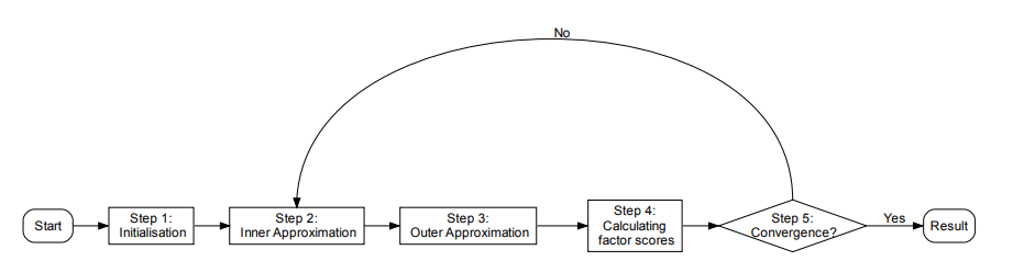
• Step1 Initialization

  각가의 LV를 MV의 가중합으로 나타낸다. 이때, MV는 표준화되어있어야 하며, 이에 따라 LV 역시 기댓값은 0이나, 표준편차가 1이 되도록 표준화를 해야한다.

  M은 MV X와 LV Y 사이의 adjacency matrix일 때, 다음과 같이 표현할 수 있다.
  \(\hat Y = XM\)
  \(\hat y_g = \frac {\hat y_g} {\sqrt {var(\hat y_g)}}\)
  

• Step2 Inner Approximation

  LV를 다른 LV의 가중합으로 나타낸다. 이때 weighting은 2.4.의 weighting scheme에 의해 계산된다. 이를 수식으로 나타내면 다음과 같다.
  \(\tilde Y = \hat Y E\)
  \(\tilde y_g = \frac{\tilde y_g }{\sqrt {var(\tilde y_g)}}\) ​
  

  이를 통해 얻는 $\tilde Y = (\tilde y_1 , \cdots , \tilde y_G)$ 를 inner estimation이라고 한다.

• Step3 Outer Approximation

  이제, 위에서 얻는 inner estimation을 이용하여 반영모델인지 형성모델인지에 따라 OLS를 적용하여 LV와 MV사이의 weights를 얻는다.

• Step4 \(\hat Y = XW\)
  \(\hat Y_g = \frac {\hat Y_g}{\sqrt {var(\hat Y_g)}}\)
  

  위와 같이 얻는 $\hat Y$ 를 새로운 outer estimator라고 한다.

  이때, $W$는 Step3에서 얻은 weights들의 행렬이다.

  
  

• Step5 수렴할 때까지 반복

2.4. Weighting Scheme

• Path Weighting Scheme

  어떤 $Y$의 element $y_i$에 대하여, $y_i$가 향하는 방향의 변수를 successor, $y_i$에 영향을 주는 변수를 predecessor라고 하자. 이때, Step2의 E는 다음과 같이 결정된다.

  
  

  \[e_{ij} = \gamma_j ~~if~~j \in ~y_i^{pred}\]

​
\(e_{ij} = corr(u_i , y_j) ~~if~~j \in ~y_i^{succ}\) ​
\(e_ij = 0 ~~~, else\)

​

2.5. Calculation of path coefficients

• 위의 PLS 알고리즘 종료 이후, path coefficients는 OLS를 통해 계산할 수 있다.