[Paper Review] A Deep Generative Approach to Conditional Sampling

1. Introduction

• 통계학과 머신러닝의 주된 주제는 $X$와 $Y$ 사이의 관계를 규명하는 것.

• 이를 $X$가 주어질 때의 $Y$의 값을 파악하는 조건부 분포(conditional distribtuion)의 문제로 이해할 수 있다.

  
  

• 본 논문에서는 조건부 분포 추정을 위해 a nonparametric generative approach to sampling from a conditional distribution을 제시한다.
  • Generative conditional distribution sampler (GCDS)
• $\eta$ 가 어떤 reference distribution에서 추출된 random variable이라 할 때, GCDS는 $G(\eta, x)$를 추정한다.

1.1. Generative Adversarial Network

• GCDS의 훈련 방법은 GAN과 비슷하다. Conditional density의 functional form을 직접 추정하는 대신, GCDS는 Conditional sampler를 추정한다. 논문에 따르면, 조건부 분포를 추정할 때 연속형 조건의 경우 모든 조건에 대해서 추정을 하는 것은 현실적으로 힘들다. 대신 각 조건에 대해서 noise를 부여하여, noise의 reference distribution와 조건 X를 반응변수 Y에 매핑시키는 conditional sampler를 추정하는 것이 더 효율적이다.

• 이러한 conditional sample 추정은 Noise outsourcing lemma에 의해 정당화된다. 이에 따르면 Conditional density estimation과 generalised nonparametric regression 문제를 동일시 할 수 있는데, 이 generalized nonparametric regression 문제가 바로 conditional sampler 추정을 의미한다.
• 예를 들어, 어떤 sampler $G(x) = G_0 (x) +\eta$를 생각하면, noise $\eta$에 따라 형성되는 sampler이며 동시에 standard nonparametric regression 문제임을 확인할 수 있다.

cGAN
$\underset{G}{argmin} \,\,\underset{D}{argmax}E_{X \sim P_X} [log D(X\vert Y) ] + E_{\eta \sim p_\eta} [log (1-D(G(X\vert Y)))]$
GCDS
$\underset{G}{argmin} \,\,\underset{D}{argmax} E_{(X,\eta ) \sim P_X, \eta} [ D(X,G(\eta, X))] - E_{(X,Y) \sim P_{X,Y}}[exp(D(X,Y))]$

1.2. pros of GCDS

1. No restirction on the dimensionality of the response variable

• 독립변수와 반응변수가 모두 고차원 이어도 추정이 가능하다.
• Image 생성과 같이 고차원 데이터도 처리할 수 있다.

2. Both continuous and discrete type variables can be dealt with

3. Easy to obtain estimates of the summary measures

• reference distribution 에서 $\eta$를 뽑아내 sampling을 할 수 있으므로, Monte Carlo를 통해 summary statistics를 쉽게 추정할 수 있다.

4. Consistency

• 생성된 샘플들은 타겟 조건부 분포에 weakly converge 한다.

1.3. Related literature

1. Smoothing method

• include kernel smoothing and local polynomials
• esimate the joint density of $(X,Y)$ and marginal density of $X$ , then get the ratio

2. Nonparametric regression

3. Nearest neighbor

• 저자는 위의 introduction 이후, 크게 세가지 스텝으로 새로운 방법론을 보이고 증명한다.
  1. 2절에서는 Noise outrsourcing lemma를 통해 nonparametric density estimation이 conditional sampler estimation으로 대체될 수 있고, 항상 그러한 conditional sampler가 존재할 수 있음을 보인다.
  2. 3절에서는 Genrative adversarial 방법론을 모델 추정에 적용하기 위해, f-divergence를 바탕으로 generator와 discriminator를 가진 Objective function을 근사한다.
  3. 4절에서는 추정된 generator가 실제의 conditional density에 점근적으로 근사(asymptotically convegent)함을 보인다.
• 이를 통해, GCDS를 통해 추정된 sample가 목표로 하는 conditional density의 추정에 사용할 수 있음을 이론적으로 보이고 있다. 그리고, 이를 바탕으로 마지막 5절에서는 실증 분석을 통해 GCDS가 실제로 활용될 가능성을 보이고 있다.

2. Generative Representation of Conditional Distribution

Notation

• $(X,Y) \in \mathcal{X} \, \times \, \mathcal{Y}$, $ \mathcal{X} \subseteq R^d $ is predictor , $ \mathcal{Y} \subseteq R^q $ response variable
• Predictor $X$ can contain both continuous and categorical components
• $\eta$ is a random variable independent of $X$ with a known distribution $P_\eta $ to be the standard normal $N(0, \mathbb{I}_m)$ for a given $ m \geq 1$

2.1. Goal of the model

• 분포 $Y ~~given ~~X=x$ 가 조건부 분포 $G (\eta , X) ~~given ~~X=x$와 같아지는 $G : \mathbb{R}^m \times \mathcal{X} \rightarrow \mathcal{Y}$ 를 찿는 것이 GCDS의 목표이다.

\[\begin{align} G( \eta , x) ~\sim ~P_{Y \vert X=x} , ~~x \in \mathcal{X} \tag{1} \end{align}\]

• 위 조건을 만족하는 $G(\eta, x)$ 를 찾을 수 있다면, reference distribution에서 $\eta$를 추출한 후 $G( \eta , x)$를 통해 $P_{Y \vert X =x}$를 얻을 수 있다.

2.2. Existence of $G(\eta, x)$

• $G$의 존재성은 noise-outsourcing lemma를 통해 증명할 수 있다.

---

Lemma 2.1. (Noise Outsourcing Lemma)

$(X,Y)$ 가 $\mathcal{X} \times \mathcal{Y}$ 상에서 joint distribution $P_{X,Y}$ 를 다르는 확률변수라고 하자. 이때, $\mathcal{X}, \mathcal{Y}$는 standard Borel space이다. 이때, $\eta \sim N(\bf{0}, \bf I)_m$ 가 $ X$와 독립이고

\[\begin{align} (X,Y) = (X, G (\eta, X)) ~~Almost ~~~Surely \tag{2} \end{align}\]

를 만족하는 $\eta$와 Borel-measurable $G : \mathbb{R}^m \times \mathcal{X} \rightarrow \mathcal{Y}$가 존재한다.

---

• 가정에 의해, $\eta$와 $X$는 독립이므로, (2) 를 만족하는 $G$는 (3)도 만족한다.

proof

​ 저자가 참고한 원문 논문에서는 $\eta \sim N(\mathbf{0}, \mathbf{I}_m)$이 아니라 $u \sim Uniform [0,1]$인 경우의 noise outsourcing lemma를 따르고 있다. (Lemma 3.1 in Austin (2015))


Basic noise outsourcing lemma에 따르면, $$ Y = G_1 (u,X) ~~almost~~~surely $$ 를 만족하는 measurable function $G_1 : [0,1] \times \mathcal{X} \rightarrow \mathcal{Y}$ 이 존재한다.


마찬가지로, 만일 $u$와 $\eta$가 독립이라면, $$ u = G_2(\eta) ~~almost ~~surely $$ 를 만족하는 measurable function $G_2 : \mathbb{R}^m \rightarrow [0,1]$이 존재한다.


따라서 이 둘을 결합 시, $$ G(\eta,x) = G_1 (G_2(\eta),x), ~~(\eta, x) \in \mathbb{R}^m \times \mathcal{X} $$ 인 $G$를 구할 수 있다.

---

• symmetry
• 
• Detecting symmetries with neural networks - IOPscience

2.3. Generalized regression problem

• Noise outsourcing lemma가 의미하는 것은 conditional distribution estimation 문제를 generalized regression 문제로 이해할 수 있다는 점이다.
• (1) 를 다르게 이해하면 다음과 같다.

\[\begin{align} Y \vert X=x ~\sim~G(\eta, x), ~~x\in \mathcal{X} \tag{3} \end{align}\]

• 즉, error가 noise $\eta$에서 나왔다고 이해하면 이는 일반적인 generalized regression 문제와 동일해진다.

• 예를 들여, $G(\eta, x) = G_0(x) + \eta$ , $E(\eta \vert X) =0$ 으로 이해하면, (3)는 전형적인 nonparametric regression 문제와 동일해진다.

  
  

2.4. a Conditional distribution, not a Unconditional distribution

• Conditional distribution을 찾는것은 unconditional distribution을 찾는 것과는 명백하게 다른 문제이다.

• GAN을 예시로 들자면, discrete condition이라면 각 condition에 대해서 distribution을 찾음으로써 conditional distribution을 추정할 수 있다. (cGAN, goodfellow et al, 2014)

• 그러나 이는 $\eta$의 함수로 만들어지는 conditional distribution을 직접 추정하는 것과는 다른 문제로, 실제로 cGAN은 continuous type random variable에 대해서는 conditional distribution 추정이 불가능하다.

  
  

• 대신, 저자는 Lemma 2.2.를 통해 $X,Y$의 Joint distribution 추정으로 conditional distribution을 추정하고자 한다.

---

Lemma 2.2.

$\eta$가 $X$와 독립이라고 하자. 이때, $G(\eta, X) \sim P_{Y \vert X=x}, x \in \mathcal{X}$와 다음은 동치이다.

\[\begin{align} (X, G(\eta, X)) \sim (X,Y) \tag{4} \end{align}\]

---

• 이는 $P_{T\vert X} = P_{Y\vert X} \quad \longleftrightarrow \quad P_{T\vert X}P_X = P_{Y\vert X}P_X $라는 사실에서 쉽게 알 수 있다.
• 따라서, (4)를 만족하는 $G$를 찾는다면, 이는 우리가 추정하고자 하는 conditional distribution이며, Monte Carlo 기법 등을 통해 $P_{Y \vert X=x}$의 summary measures 역시 추정할 수 있다.

\[\begin{align} \tilde{g}(x) = \frac{1}{J} \sum_{j=1}^J G(\eta_j ,x) ~~and ~~ \tilde{v}(x) = \frac{1}{J} \sum_{j=1}^J [G(\eta_j ,x) - \tilde{g}(x)]^2 \tag{5} \end{align}\]

3. Distribution Matching Estimation

3.1. f-divergence and its variational form

---

​ Lemma 3.1. Let $\mathcal{D}$ be a class of measurable function $D : \mathbb{R}^d \rightarrow \mathbb{R}$. Suppose $f$ is a differentiable convex function. Then,

\[\begin{align} \mathbb{D}_f (q \vert \vert p) \geq \underset{D \in \mathcal{D}}{sup} [\mathbb{E}_{Z\sim q}D(Z) - \mathbb{E}_{W \sim p} f^* (D(W))] \tag{B.1} \end{align}\]

where the equality holds if and only if $f’(q/p) \in \mathcal{D}$ and the supreme is attained at $D^* =f’ (q/p)$ .

proof)

definition) Fenchel conjugate of f $$ f^*(t) = \underset{x \in \mathbb{R}}{sup} \{ tx - f(x) \} , t \in \mathbb{R} $$ If f is convex function, $f^{**} = f$. First, $f^{**} \leq f$ $$ \begin{align} f^{**}(t) & = \underset{s \in \mathbb{R}}{sup} \{ st - \underset{s \in \mathbb{R}}{sup}\} \{ st - f^*(s) \}\\ &= \underset{s \in \mathbb{R}}{sup} \{ st - \underset{x \in \mathbb{R}}{sup} \{ tx - f(x) \}\} \\ &= \underset{s \in \mathbb{R}}{sup} ~ \underset{x \in \mathbb{R}}{inf} \{ s(t-x) + f(x)\} \\& \leq \underset{x \in \mathbb{R}}{inf} ~\underset{s \in \mathbb{R}}{sup} \{s(t-x) + f(x)\} = f(t) \end{align} $$ Second, if $f$ is convex, there is no $f$ such that $f^{**} < f$. Hyperplane separation theorem is needed for the contradiction, I will skip it. By fermat's rule, the maximizer $s^*$ satisfies $$ t \in \partial f^* (s^*) \longleftrightarrow s^* \in \partial f(t) $$ One can obtain Lemma 3.1. by applying above result to definition of f-divergence.

---

3.2. Distribution matich estimation via f-divergence

Now to construct objective function, consider the KL divergence below.

\[\mathbb{D}_{KL} (p_{X,G(\eta, X)} \vert \vert P_{X,Y} ) = \mathbb{E}_{(X,\eta) \sim P_{X,\eta}} [ log ~r(X,G(\eta, X))], ~~~where ~r(z) = \frac{p_{X,G(\eta,X)} (z)}{p_{X,Y}(z)}\]

Here, the authors suggest to use $D=log ~r$ as a discriminator, since $r$ means the ratio of generator and real data.

Since the conjugacy of $f(x) = x ~logx$ is $f^* (t) = exp(t-1)$, using lemma 3.1,

\[\begin{align} \mathbb{D}_{KL} (p_{X,G(\eta, X)} \vert \vert P_{X,Y} ) &= \mathbb{E}_{(X,\eta) \sim P_{X,\eta}} [ log ~r(X,G(\eta, X))]\\ &= \underset{D}{sup} \{ \mathbb{E} _{(X, \eta) \sim P_X P_\eta}[D(X,G(\eta, X)] - \mathbb{E} _{(X,Y) \sim P_{X,Y} }[ exp(D(X,Y) -1]\}\\ &= \underset{D}{sup} \{ \mathbb{E} _{(X, \eta) \sim P_X P_\eta}[D(X,G(\eta, X)] - \mathbb{E} _{(X,Y) \sim P_{X,Y} }[ exp(D(X,Y)]\} +1\\ &\approx \underset{D}{sup} \{ \mathbb{E} _{(X, \eta) \sim P_X P_\eta}[D(X,G(\eta, X)] - \mathbb{E} _{(X,Y) \sim P_{X,Y} }[ exp(D(X,Y)]\} \end{align}\]

First equality holds because $x ~logx$ is measurable function. Approximation is used since constant does not affect the result.

Therefore, we can summarise the objective function approximated to :

\[\mathcal{L} (G,D) = \mathbb{E} _ {(X, \eta) \sim P_X P_\eta} [D(X,G(\eta, X))] - \mathbb{E} _ {(X, Y) \sim P_{X,Y}}[exp(D(X,Y)]\]

, Which means that

\[\underset{G}{argmin} \,\,\underset{D}{argmax} E_{(X,\eta ) \sim P_X, \eta} [ D(X,G(\eta, X))] - E_{(X,Y) \sim P_{X,Y}}[exp(D(X,Y))]\]

4. Weak Convergence of Conditional Sampler

4.1. Notation

• 증명을 시작하기에 앞서, 몇가지 노테이션을 정리한다.

\[\begin{align} \mathbb{L}(G) = \underset{D} {sup} \mathcal{L} (G,D) \tag{C.1} \end{align}\]

,라 할 때, Lemma3.1. **에 의해 **sup을 만족하는 $D$는 $f’(q/p) = 1 + logx \approx D $에 의해 $log ~\frac{P_{XG}(z)}{P_{XY}(z)} = log ~r(z)$ 이다.

\[\begin{align} D^* (z) =log ~\frac{P_{XG}(z)}{P_{XY}(z)} = log ~r(z) \tag{C.2} \end{align}\]

• 따라서, Generator가 영향을 주지 않는 부분을 제하면

\[\begin{align} \mathbb{L}(G) = \mathbb{E} _ {(X, \eta) \sim P_X P_\eta} [log ~r(X,G(\eta, X))] \tag{C.3} \end{align}\]

가 성립하며, Lemma 2.2. 에 의해 이를 극소화하는 $G^*$는 $P_{Y\vert X}$가 된다.

\[\begin{align} G^\star (\eta, X) \sim P_{Y \vert X=x}, x \in \mathcal{X} \tag{C.4} \end{align}\]

• Empirically, 이는 다음과 같이 표현한다.

\[\begin{align} \mathbb{\hat{L}}(G) &= \underset{D_\phi \in \mathcal{D}} {sup} \mathcal{\hat{L}} (G,D) \tag{C.5} \\ \hat{G}_\theta \in arg &~min _ {G_\theta \in \mathcal{G}} \hat{\mathcal{L}}(G_\theta , \hat{D_\phi}) \tag{C.6} \\ \hat{D}_\phi \in arg &~min _ {D_\phi \in \mathcal{D}} \hat{\mathcal{L}}(\hat{G_\theta} , {D_\phi}) \tag{C.7} \end{align}\]

4.2. Assumptions

(A1) The target conditional genearator $ G^\star: \mathbb{R}^m \times \mathcal{X} \rightarrow \mathcal{Y} $ is continuous with $\vert \vert G^\star \vert \vert_\infty \leq C_0$ for some constant $0<C_0 <\infty$

(A2) For any $G \in \mathcal{G} $ , $r_G (z) = \frac{p_{X,G(\eta,X)}(z)}{p_{X,Y}(z)}$ : $\mathcal{X} \times \mathcal{Y} \rightarrow \mathbb{R}$ is continuous and $0<C_1 \leq r_G (z) \leq C_2$

• 위의 두가지 가정은 conditional density estimation에서 많이 사용되는 가정이며, 현실적으로 가정하기에 무리는 없다.

• 추가적으로, 훈련에 사용되는 신경망 $G,D$에 대해 다음의 가정을 추가한다.

depth $\mathcal{H}$ : number of hidden layers

width $\mathcal{W}$ : $max\,\,{w_1 , \cdots , w_\mathcal{H}}$ for $w_i$ is width of $i$th layer

size $\mathcal{S}$ : $\sum_{i=0}^{\mathcal{H}} [w_i \times (w_i +1)]$ is the total number of parameters in the network.

bound $\mathcal{B}$ : $\vert \vert G \vert \vert_\infty \leq \mathcal{B}$ is the bound of neural network

(N1) The network parameters of $\mathcal{G}$ satisfies \(\mathcal{H} \mathcal{W} \rightarrow \infty ~~and~~ \frac{\mathcal{B} \mathcal{S} \mathcal{H} log(\mathcal{S}) logn}{n} \rightarrow 0, ~~as ~~n \rightarrow\infty\)

(N2) The network parameters of $\mathcal{D}$ satisfies \(\tilde{\mathcal{H}} \tilde{\mathcal{W}} \rightarrow \infty ~~and~~ \frac{\tilde{\mathcal{B}} \tilde{\mathcal{S}} \tilde{\mathcal{H}} log(\tilde{\mathcal{S}}) logn}{n} \rightarrow 0, ~~as ~~n \rightarrow\infty\)

• 이들 가정 역시 충분히 현실적인 가정인데, 표본 수가 무한하게 많아진다면 그만큼 뉴럴네트워크가 커져야하며, 동시에 표본의 증가속도보다는 뉴럴네트워크의 크기 확장속도가 작아야 한다.

4.3. Total Variation norm convergence

---

Theorem 4.1. 위의 조건들이 만족될 때, 다음이 성립한다.

\[\begin{align} { \large \mathbb{E}_{(X_i, Y_i , \eta_i)_{i=1}^n } \vert \vert p_{X, \hat{G}_\theta (\eta, X)} - p_{X,Y} \vert \vert _{L_1}^2 \rightarrow 0 , ~~as ~n \rightarrow 0 } \tag{C.8} \end{align}\]

• 해당 부분의 proof가 길기 때문에, proof를 여러 부분으로 나누어서 설명.

---

proof1

​ Pinsker's theorem과 $\mathbb{L} (G^\star) =0$에 의해 $ \vert \vert p_{X, \hat{G}_\theta (\eta, X)} - p_{X,Y} \vert \vert _{L_1}^2$는 다음이 성립한다. $$ \begin{align} \vert \vert p_{X, \hat{G}_\theta (\eta, X)} - p_{X,Y} \vert \vert _{L_1}^2 \leq 2(\mathbb{L}(\hat{G}) - \mathbb{L}(G^*)) \tag{C.9} \end{align} $$

- Pinkser's theorem if $P$ and $Q$ are probability densities defined on a measurable space $(X, \Omega)$, $$ \vert \vert P-Q \vert \vert_{L_1} \leq \sqrt{2D_{KL}(P \vert \vert Q)} $$

따라서, 어떠한 generator $\bar{G} \in \mathcal{G}$ 에 대하여, $\mathbb{L}(\hat{G}) - \mathbb{L}(G^*)$ 는 다음을 만족한다. $$ \begin{align} \mathbb{L}(\hat{G}) - \mathbb{L}(G^\star) &= \underset{D}{sup} \mathcal{L}(\hat{G},D) - \underset{D\in \mathcal{D}}{sup} \mathcal{L}(\hat{G},D) \tag{C.10} \\ &+ \underset{D\in \mathcal{D}}{sup} \mathcal{L}(\hat{G},D) - \underset{D\in \mathcal{D}}{sup} \mathcal{\hat{L}}(\hat{G},D) \tag{C.11} \\ & +\underset{D\in \mathcal{D}}{sup} \mathcal{\hat{L}}(\hat{G},D)-\underset{D\in \mathcal{D}}{sup} \mathcal{\hat{L}}(\bar{G},D) \tag{C.12} \\ & +\underset{D\in \mathcal{D}}{sup} \mathcal{\hat{L}}(\bar{G},D)-\underset{D\in \mathcal{D}}{sup} \mathcal{L}(\bar{G},D) \tag{C.13} \\&+ \underset{D\in \mathcal{D}}{sup} \mathcal{L}(\bar{G},D) - \underset{D}{sup} \mathcal{L}(\bar{G},D) \tag{C.14} \\ &+ \underset{D}{sup} \mathcal{L}(\bar{G},D) - \underset{D}{sup} \mathcal{L}(G^\star,D) \tag{C.15} \end{align} $$

이때, $(C.12), (C.14)$는 0보다 크거나 같고, $(C.11), (C.13)$은 $\underset{D \in \mathcal{D}, G \in \mathcal{G}}{sup} \vert\mathcal{L} (G,D) - \hat{\mathcal{L}}(G,D)\vert$보다 작으므로, 다음이 성립한다. $$ \begin{align} \mathbb{L}(\hat{G}) - \mathbb{L}(G^\star) &\leq \underset{D}{sup} \mathcal{L}(\hat{G},D) - \underset{D\in \mathcal{D}}{sup} \mathcal{L}(\hat{G},D) \\ & +2 \underset{D \in \mathcal{D}, G \in \mathcal{G}}{sup} \vert\mathcal{L} (G,D) - \hat{\mathcal{L}}(G,D)\vert\\ & + \underset{D}{sup} \mathcal{L}(\bar{G},D) - \underset{D}{sup} \mathcal{L}(G^\star,D) \\& \equiv \triangle_1 + \triangle_2 + \triangle_3 \end{align} $$ 이때 $\triangle_{1}, \triangle_{3}$는 근사오류(approximation error)이며 $\triangle_{2}$는 통계적 오류(Statistical error)라고 할 수 있다.

---

more lemmas for proof

Lemma B.4. if $\xi _i ~~,i = 1, \cdots ,m $ are $m$ finite linear combinations of Rademacher variables $\epsilon_j, ~~j = 1, \cdots ,J$. Then, $$ \mathbb{E}_{\epsilon_j , j=1, \cdots,J} \underset{1\leq i \leq m}{max} \vert \xi_i \vert \quad\leq \quad C (log \, m )^{\frac{1}{2}} \underset{1 \leq i \leq m}{max} (\mathbb{E} \xi_i^2 )^{\frac{1}{2}} $$ for some constant $C >0$

proof) This result follows from Corollary 3.2.6 and inequality 4.3.1 in De la Pena and Gine (2012) with $\Phi(x) = exp(x^2)$

---

Lemma B.5. Let $f$ be a uniformly continuous function defined on $E \in [-R,R]^d$. For arbitrary $L \in \mathbb{N}^+$ and $N \in \mathbb{N}^+$, there exists a function $ReLU$ network $f_\phi$ with width $3^{d+3} max\{d \lfloor{N^{1/d} }\rfloor, N+1 \} $ and depth $12L + 14 + 2d$ such that $$ \vert \vert f - f_\phi \vert \vert_{L^\infty (E)} \leq 19 \sqrt{d} \omega_f ^E (2RN^{-2/d} L^{-2/d}) $$ where, $\omega_f^E (t)$ is the modulus of continuity of $f$ satisfying $\omega_f^E (t) \rightarrow 0$ as $t \rightarrow 0^+$

proof can be found on Theorem 4.3. in Shen et al.(2020)

---

proof of error3

Lemma B.1. $$ \begin{align}\triangle_3 \equiv inf_{\bar{G} \in \mathcal{G}} [\mathbb{L}(\bar{G}) - \mathbb{L}(G^\star )] = o(1), ~~as ~~n \rightarrow \infty \tag{D.1.} \end{align} $$

proof) 가정 A1에 의해 $G^\star$은 $E_1 = [-B, B]^{d+m}, ~~B = log \,n$에서 연속이고, $\vert \vert G^\star \vert \vert _{L^\infty} \leq C_0 ~~for ~~some ~~C_0 \geq0$가 성립한다. $L= log \, n ,~N = \frac{n^{\frac{d+m}{2(2+d+m)}}}{log \, n} ~, E=E_1 ,~ R=B $로 보면, Lemma B.5. 에 의해 아래 (D.2.)를 만족하는 ReLU network $\bar{G}_\bar{\theta} \in \mathcal{G}$를 찾을 수 있다.
$$ \begin{align} \vert \vert G^\star - \bar{G}_\bar{\theta} \vert \vert_{L^\infty (E_1)} \leq 19 \sqrt{d+m} \omega_F^{E_1} (2 (log \, n) n^{\frac{-1}{2+d+m}}) \tag{D.2.} \end{align} $$
, 이때, $\bar{G}_\bar{\theta}$는 $depth ~~\mathcal{H} = 12log\,n +14 +2(d+m)$,
$width ~~\mathcal{W} = 3^{d+m+3} max\{ (d+m) (\frac{n^{\frac{d+m}{2(2+d+m)}}}{log \, n})^{\frac{1}{d+m} } , \frac{n^{\frac{d+m}{2(2+d+m)}}}{log \, n} +1\}$,
$size ~~\mathcal{S} = \frac{n^{\frac{d+m-2}{d+m+2}}}{log^4 n}$ 의 네트워크 구조를 가지는 네트워크를 의미한다.

또한 $\bar{D} = log {\frac {p_{X,\bar{G}_{\bar{\theta}\,(\eta, X)}(z)}}{p_{X,Y}(z)}}$ , $D^\star = log {\frac {p_{X,G^\star_{\bar{\theta}\,(\eta, X)}(z)}}{p_{X,Y}(z)}}$으로 $G$의 함수이고 가정에 의해 $G$는 continuity를 만족하므로, $\vert \vert D^* - \bar{D}\vert \vert \rightarrow 0 $ 역시 만족된다.
따라서,
$$ \mathbb{L} (\bar{G}) = \underset{D}{sup} \mathcal{L}(\bar{G} ,D) = \mathbb{E} _ {(X, \eta) \sim P_X P_\eta} [\bar{D}(X,\bar{G}(\eta, X))] - \mathbb{E} _ {(X, Y) \sim P_{X,Y}}[exp(\bar{D}(X,Y)] $$
는 $n \rightarrow \infty$에 따라
$$ \mathbb{L} (G^\star) = \underset{D}{sup} \mathcal{L}(G^\star ,D) = \mathbb{E} _ {(X, \eta) \sim P_X P_\eta} [D^\star(X,G^\star(\eta, X))] - \mathbb{E} _ {(X, Y) \sim P_{X,Y}}[exp(D^\star(X,Y)] $$ 에 수렴한다.

---

proof of error2

Lemma B.2.
$$ \begin{align} \triangle_2 \equiv \underset{D \in \mathcal{D} ,G \in \mathcal{G}}{sup} \vert \mathcal{L} (G,D) - \hat{\mathcal{L}}(G,D) \vert \leq \mathcal{O} (n^{\frac{-2}{2+d+m}} +n^{\frac{-2}{2+d+q}} ) \tag{D.3.} \end{align} $$
proof) 다음과 같은 노테이션을 정한다.
- $Z = (X,Y) \sim P_{X,Y}$ and $Z_i = (X_i, Y_i), ~i = 1,\cdots,n$ are $i.i.d.$ copies of $Z$
- $\eta \sim P_\eta$ and $\eta_j,~j =1, \cdots, n$ are $i.i.d.$ copies of $\eta$ , $\eta \perp X$
- $W_i = (X_i , \eta_i) $ are $i.i.d.$ copies of $W = (X , \eta) \sim P_{X}P_{\eta}$
- $S = (W,Z) \sim (P_X P_\eta) \otimes P_{X,Y}$ and $S_i = (W_i, Z_i) = ((X_i, \eta_i), (X_i, Y_i)), ~~i = 1,\cdots,n$ are $i.i.d.$ copies of $S$.
- $b(G,D;S) = D(X,G(\eta,X)) - exp(D(X,Y))$
- $\mathcal{L}(G,D) = \mathbb{E}_{S} [b(G,D, ;S)]$
- $\hat{\mathcal{L}}(G,D) = \frac{1}{n} \sum_{i=1}^n b(G,D, ;S)$
- $\epsilon_i , ~~i = 1, \cdots ,n $ 를 $S_i$와 독립인 Rademacher 확률변수라고 하면, Rademacher complexity of $\mathcal{D} \times \mathcal{G}$를 다음과 같이 정의한다.
$$ \begin{align} \mathcal{C}(\mathcal{D} \times \mathcal{G}) = \frac{1}{n} \mathbb{E}_{\{S_i, \epsilon_i\}_{i=1} ^n } \left[ \underset{G \in \mathcal{G}, D\in \mathcal{D} }{sup} \left\vert \sum_{i=1}^n \epsilon_i b(G,D, ;S) \right\vert \right] \tag{D.4.} \end{align} $$
이제, symmetrization technique과 law of iterated expectation을 이용하면 다음을 보일 수 있다.
$$ \begin{align} &\underset{D \in \mathcal{D} ,G \in \mathcal{G}}{sup} \vert \mathcal{L} (G,D) - \hat{\mathcal{L}}(G,D) \vert \\ &= \underset{D \in \mathcal{D} ,G \in \mathcal{G}}{sup} \vert \mathbb{E}_S b(G,D,S)- \frac{1}{n} \sum_{i=1}^n b(G,D; S_i') \vert ~~\longleftarrow S_i'\,\,\,is\,\,\,i.i.d. \,\,\,copy\,\,\,of\,\,\,S_i \\ &=\underset{D \in \mathcal{D} ,G \in \mathcal{G}}{sup} \left\vert \mathbb{E}_S \left[\frac{1}{n}\sum_{i=1}^n (b(G,D,S_i )- b(G,D; S_i'))\right] \right\vert \\ & \leq \mathbb{E}_{S,S'} \left[ \underset{D \in \mathcal{D} ,G \in \mathcal{G}}{sup} \left\vert \frac{1}{n}\sum_{i=1}^n (b(G,D,S_i )- b(G,D; S_i')) \right\vert \right] \\ &= \mathbb{E}_{S,S', \epsilon} \left[ \underset{D \in \mathcal{D} ,G \in \mathcal{G}}{sup} \left\vert \frac{1}{n}\sum_{i=1}^n \epsilon_i (b(G,D,S_i )- b(G,D; S_i')) \right\vert \right] \\ &\leq 2\mathbb{E}_{S, \epsilon} \left[ \underset{D \in \mathcal{D} ,G \in \mathcal{G}}{sup} \left\vert \frac{1}{n}\sum_{i=1}^n \epsilon_i b(G,D,S_i ) \right\vert \right] \\ &= 2\mathcal{C}(\mathcal{D} \times \mathcal{G})\\ &= 2 \mathbb{E}_{S_1, \cdots, S_n} \left\{ \mathbb{E}_{\epsilon_1 , \cdots, \epsilon_n} \left[ \underset{G \in \mathcal{G}, D\in \mathcal{D} }{sup} \left\vert \frac{1}{n}\sum_{i=1}^n \epsilon_i b(G,D, ;S_i) \right\vert \vert S_1 , \cdots, S_n \right] \right\} \tag{D.5.} \end{align} $$
어떤 $\delta >0$에 대하여, $\mathcal{D}_{\delta} \times \mathcal{G}_{\delta}$ 를 $\mathcal{D} \times \mathcal{G}$의 $\delta - cover$라 하고, $\scr{C}(\cal{D} \times \cal{G}, e_{n,1}, \delta )$를 다음의 empirical distnace $e_{n,1}$을 distance로 가지는 covering set이라고 하면,
$$ e_{n,1}((G,D), (\tilde{G}, \tilde{D})) = \frac{1}{n} \mathbb{E}_\epsilon \left[ \sum_{i=1}^n \left\vert\epsilon_i (b(G,D;S_i) - b(\tilde{G}, \tilde{D}; S_i)) \right\vert\right] $$
또한, 가정 A1, A2에 의해 $b(G,D;S_i)$ 가 어떤 수에 의해 bounded 되므로, $b(G,D;S_i) < C_4$라 하고, Lemma B.4. 와 함께 적용 시 다음 결과를 얻을 수 있다.
$$ \begin{align} &\mathbb{E}_{S_1, \cdots, S_n} \left\{ \mathbb{E}_{\epsilon_1 , \cdots, \epsilon_n} \left[ \underset{G \in \mathcal{G}, D\in \mathcal{D} }{sup} \left\vert \frac{1}{n}\sum_{i=1}^n \epsilon_i b(G,D, ;S_i) \right\vert \vert S_1 , \cdots, S_n \right] \right\} \\ &\leq \delta + \frac{1}{n} \mathbb{E}_{S_1, \cdots, S_n} \left\{ \mathbb{E}_{\epsilon_1 , \cdots, \epsilon_n} \left[ \underset{G \in \mathcal{G_\delta}, D\in \mathcal{D_\delta} }{sup} \left\vert \sum_{i=1}^n \epsilon_i b(G,D, ;S_i) \right\vert \vert S_1 , \cdots, S_n \right] \right\} ~~\longleftarrow ~~ by ~~definition ~~of~~covering~~\delta - cover\\ &\leq 2 \delta + C_5 \frac{1}{n}\mathbb{E}_{S_1 ,\cdots ,S_n } \left\{ \left[ log \scr{C} (\mathcal{D} \times \cal{G} , e_{n,1} , \delta )\right]^{1/2} \underset{(G,D) \in \mathcal{D_\delta} \times \mathcal{G_\delta}}{max} \left[ \sum_{i=1}^n b^2(G,D ; S_i)\right]^{1/2} \right\} \\ & \leq 2 \delta + C_5 \frac{1}{n}\mathbb{E}_{S_1 ,\cdots ,S_n } \left\{ \left[ log \scr{C} (\mathcal{D} \times \cal{G} , e_{n,1} , \delta )\right]^{1/2} \sqrt{n}C_4 \right\} ~~~~~~~~~~~~~~~~~~~~~~~~~~~~~~\longleftarrow ~~by~~\left[ \sum_{i=1}^n b^2(G,D ; S_i)\right]^{1/2} \leq \sqrt{n}C_4 \\ &\leq2 \delta + C_6 \frac{1}{\sqrt{n}} \left[ log \scr{C} (\mathcal{D} , e_{n,1} , \delta ) + log \scr{C} (\cal{G} , e_{n,1} , \delta )\right]^{1/2} ~~~~~~~~~~~~~~~~~~~~~~~~~~~~~~\longleftarrow ~~ by ~~definition ~~of~~covering~~\delta - cover\\ &\leq 2\delta + C_6 \frac{1}{\sqrt{n}} \left[ log \scr{C} (\mathcal{D} , e_{n,\infty} , \delta ) + log \scr{C} (\cal{G} , e_{n,\infty} , \delta )\right]^{1/2}~~~~~~~~~~~~~~~~~~~~~~~~~~~\longleftarrow ~~by ~~e_{n,\infty} \leq e_{n,1} \tag{D.6.} \end{align} $$ 또한 위의 definition 하에서 neural network $G,D$에 대해 다음이 만족된다.
$$ og \mathscr{C} (\mathcal{D} , e_{n,\infty} , \delta ) \leq \mathcal{P}dim_\mathcal{G}~log \frac{2e \mathcal{B}n}{\mathcal{P}dim_\mathcal{G}} $$ $\mathcal{P}dim$은 PseudoDimension 이며, 다음을 만족한다.
$$ C_7 \mathcal{H}\mathcal{S} log \mathcal{S} \leq\mathcal{P}dim \leq C_8 \mathcal{H}\mathcal{S} log \mathcal{S} $$ 따라서, (D.6.) 는 다음을 따름을 보일 수 있다.
$$ C_6 \frac{1}{\sqrt{n}}\left[ log \scr{C} (\mathcal{D} , e_{n,\infty} , \delta ) + log \scr{C} (\cal{G} , e_{n,\infty} , \delta )\right]^{1/2} \leq C_9 \frac{1}{\sqrt{n}}\left[ \mathcal{H}\mathcal{S} log \,\mathcal{S} log \frac{\mathcal{B} n }{\mathcal{H}\mathcal{S} log \,\mathcal{S}} + \mathcal{\tilde{H}}\mathcal{\tilde{S}} log \,\mathcal{\tilde{S}} log \frac{\mathcal{\tilde{B}} n }{\mathcal{\tilde{H}} \mathcal{\tilde{S}} log \,\mathcal{\tilde{S}}} \right]^{1/2} $$ 위의 결과를 정리 후 N1, N2 가정과 $\delta= \frac{1}{n}$을 가정 시 다음 결과에 도달한다.
$$ \underset{D \in \mathcal{D} ,G \in \mathcal{G}}{sup} \vert \mathcal{L} (G,D) - \hat{\mathcal{L}}(G,D) \vert \leq 2 \left(2 \delta + C_9 \frac{1}{\sqrt{n}}\left[ \mathcal{H}\mathcal{S} log \,\mathcal{S} log \frac{\mathcal{B} n }{\delta \mathcal{H}\mathcal{S} log \,\mathcal{S}} + \mathcal{\tilde{H}}\mathcal{\tilde{S}} log \,\mathcal{\tilde{S}} log \frac{\mathcal{\tilde{B}} n }{\delta \mathcal{\tilde{H}} \mathcal{\tilde{S}} log \,\mathcal{\tilde{S}}} \right]^{1/2} \right) \rightarrow 0 \tag{D.7.} $$

---

proof of error1

Lemma B.3.
$$ \begin{align} \mathbb{E}_{(X_i ,Y_i, \eta_i )_{i=1}^n } [ \triangle_1 ] \equiv \mathbb{E}_{(X_i ,Y_i, \eta_i )_{i=1}^n } [\underset{D}{sup} \mathcal{L}(\hat{G},D) - \underset{D\in \mathcal{D}}{sup} \mathcal{L}(\hat{G},D)] \rightarrow 0 \tag{D.8.} \end{align} $$ $\underset{D}{sup} \mathcal{L}(\hat{G},D)$는 Lemma B.2. 에 의해 $\mathcal{L}(\hat{G},D_{\hat{G}} ),~~ where ~~ D_\hat{G} (z) =log ~\frac{P_{X\hat{G}}(z)}{P_{XY}(z)} = log ~r(z)$에서 달성된다. 가정 A1, A2에 의해 $D_\hat{G} (z) $ 는 $E_2 = [-B,B]^{d+q}, ~~B = lon \, n$ 에서 연속적이며 $\vert \vert D_\hat{G} \vert \vert_{L^\infty} \leq C_3$를 만족한다. error3의 증명 과정과 유사하게, $L= log \, n ,~N = \frac{n^{\frac{d+q}{2(2+d+q)}}}{log \, n} ~, E=E_2 ,~ R=B $로 보면, Lemma B.5. 에 의해 아래 (D.9.) 만족하는 ReLU network $D_\hat{G} \in \mathcal{D}$를 찾을 수 있다.
$$ \begin{align} \vert \vert D_\hat{G} - \hat{D}_\phi \vert \vert_{L^\infty (E_2)} \leq 19 \sqrt{d+q} \omega_F^{E_2} (2 (log \, n) n^{\frac{-1}{2+d+q}}) \label{eq:D_ninth} \tag{D.9.} \end{align} $$ , 이때, $\bar{D}_\bar{\phi}$는 $depth ~~\tilde{\mathcal{H}} = 12log\,n +14 +2(d+q)$,
$width ~~\tilde{\mathcal{W}} = 3^{d+q+3} max\{ (d+q) (\frac{n^{\frac{d+q}{2(2+d+q)}}}{log \, n})^{\frac{1}{d+q} } , \frac{n^{\frac{d+q}{2(2+d+q)}}}{log \, n} +1\}$,
$size ~~\tilde{\mathcal{S}} = \frac{n^{\frac{d+q-2}{d+q+2}}}{log^4 n}$ 의 네트워크 구조를 가지는 네트워크를 의미한다.

따라서, continuity에 의해,
$$ 0<\underset{D}{sup} \mathcal{L}(\hat{G},D) - \underset{D\in \mathcal{D}}{sup} \mathcal{L}(\hat{G},D) \leq \mathcal{L}(\hat{G},D_{\hat{G}} ) - \mathcal{L} (\hat{G} - \hat{D}_\phi) \rightarrow 0 $$ 가 성립한다.

---

5. experiments

5.1. Simulation studies

For the finite sample performance of GCDS, the authors compared the model with 3 previous methods, including the nearest neighbor kernel conditional density estimation (NNKCDE, Dalmasso et al. (2020)), the conditional kernel density estimation (CKDE, implemented in the R package np, Hall et al. (2004)), and the basis expansion method FlexCode (Izbicki et al., 2017)).

Mean and SD are estimated by Monte Carlo for GCDS. For other methods, numerical integration is used for calculation. For GCDS, conditional density is estimated using the samples generated from GCDS with kernel smoothing.

Table1 : MSE of the estimated conditional mean, estimated standard deviation

Figure1 :Comparison of density estimation

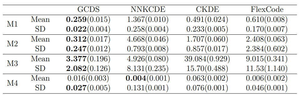
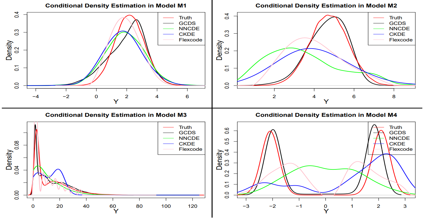
We see that GCDS yields smaller MSEs for estimation conditional mean and SD in most cases. Density plots show that GCDS yields better conditional density estimates than others. Especially, DCGS shows that it can follow multi modal densities well.

5.2. MNIST handwrittened digit

Another viewpoint for DCGS is that it can handle high-dimensional data problems as well. MNIST data is example. The images are stored in 28$\times$28 matrices with gray color intensity from 0 to 1. Each image is paired with a label in {0,1, … , 9}. The authors performed two tasks: generating images from labels and reconstructing the missing part of an image.

Generating images from label

Like a standard conditional GAN, the authors input labels $[1, 0, .., 0 ] \sim [0, … , 1]$ as a condition. The results are like below figure 2.

Figure2 : Left one is real data, right one is generated data

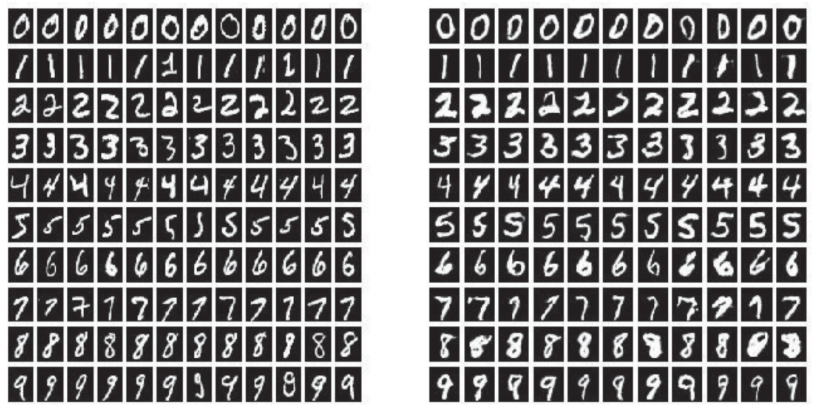
It is easy to see that generated image is similar to real image. Also, for each label, generated images are all different because of noise input. However, it is not especially different from conditional GAN method.

Reconstructing the missing part of an image

Special part of DCGS is that it can adopt ‘continuous condition’, which is not possible for standard GAN. Reconstructing the missing part of an image is an example.

Figure3 : Reconstruction of missing part

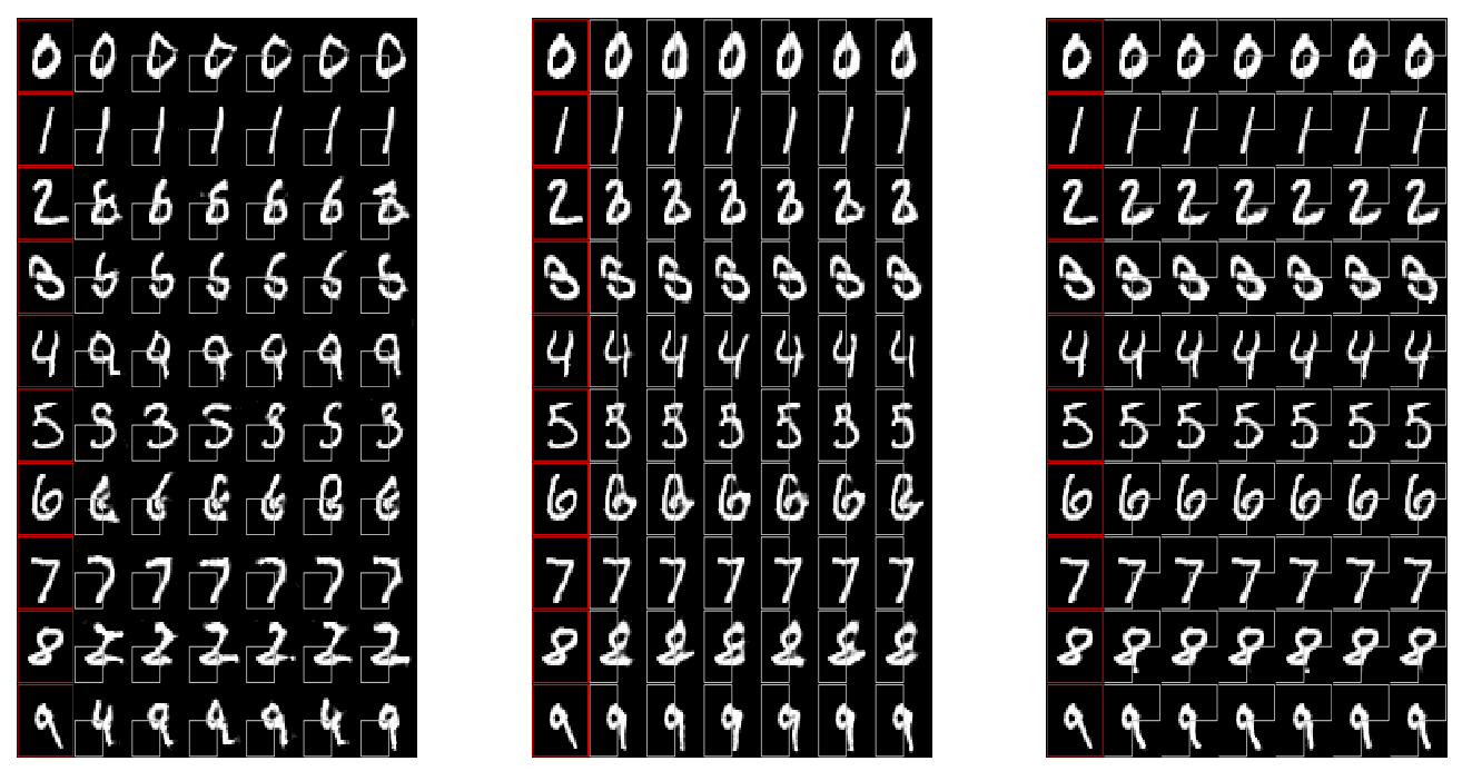
Reconstructed images given partial image in MNIST dataset. The first column in each panel consists of the true images, the other columns give the constructed images. In the left panel, the left lower 1/4 of the image is given; in the middle panel, the left 1/2 of the image is given; in the right panel, 3/4 of the image is given.

Here, image is conditions, which are high-dimensional conditional data. It is not available for standard GAN method. Also, when 1/4 of image is given, It does not show good reconstruction quality. However, as more part of image is given, reconstruction quality increases. Therefore, it shows that GCDS can take high-dimensional data, with continuous or discrete columns, could be handle for both predictors and responses.