[Paper Review]Generative Adversarial Networks
- Generative Adversarial Networks is a paper by Ian Goodfellow in 2014.
It is cited 44,776 times, one of the most cited papers.
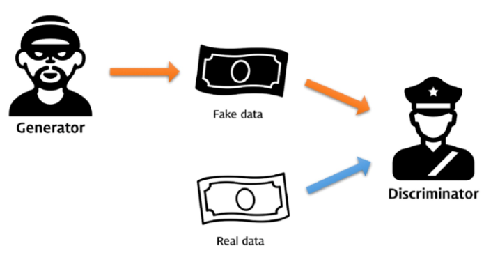
- Goodfellow suggested a miracle generative framework, made by competition between the generative model and discriminative model
1) generative model , G: make data according to distribution somewhat similar to real data distribution , trying to real fake data that discriminator cannot distinguish
2) discriminative model, D: Try to discriminate the fake data from the generative model as fake.
1. Introduction
- Deep learning tries to find out the distribution of population data. It uses a ton of linear & nonlinear functions for the approximation, based on backpropagation and dropout algorithm
- However, deep generative models did not have success
- Goodfellow suggested a generative framework, made by competition between the generative model and discriminative model
- He has examples of counterfeit money makers and police officers. The criminal tries to make a perfect counterfeit to cheat the police officer, on the other side, the police officer tries to find what is counterfeit. In the process.
2. Adversarial nets
-
Many different kinds of methodology could be used for training, but multiplayer perceptron is the most straightforward.
-
$min_G$ $max_D V(D,G) = E_{x \sim p_{data}(x)} [log D(x)] + E_{z \sim p_z (z) } [log(1-D(G(z)))] $
-
$P_{data}(x)$ : sample $x$ from real data distribution
And, $p_{Z} (z)$ : sample latent code z from Gaussian distribution
-> classify real as real (: $D(x)\sim 1$)
-> classify fake as fkae(: $D(G(z)) \sim 0$)
3. Theoretical result
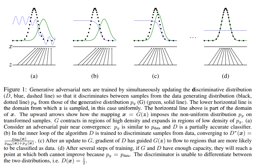
- For gan to work well, we need that: $p_g $of generator should converge to $p_{data}$, that is, a generator should generate data somewhat similar to real data
- 3.1. really show that $p_g = p_{data}$ is true, and 3.2. shows that algorithm 1 is the way to realize minimax problem
3.1. $p_g = p_{data}$
-
proposition 1
$max_D V(D,G) = E_{x \sim p_{data}(x)} [log D(x)] + E_{z \sim p_z (z) } [log(1-D(G(z)))] $ attain global minimum at $p_G = p_{data}$
-
$min_G$ $max_D V(D,G) = E_{x \sim p_{data}(x)} [log D(x)] + E_{z \sim p_z (z) } [log(1-D(G(z)))] $
=(change of variables) $min_G$$max_D V(D,G) = E_{x \sim p_{data}(x)} [log D(x)] + E_{x \sim p_G } [log(1-D(x))] $
=(expectation) $min_G$ $\int_X max_D (V(D,G) = p_{data} (x) [log D(x)] +p_G (x) [log(1-D(G(z)))] )dx $
$~~$
- if $f(y) = a log y + blog (1-y) $
$f’(y) = \frac{a}{y} - \frac{b}{1-y} , ~~~ f’(y)=0 <-> y= \frac{a}{a+b } (local ~ max)$
$~$
-
Optimal discriminatro : $D_g ^* (x) = \frac{p_{data} (x)}{p_{data}(x) + p_G (x) }$
Putting it back into the equation,
= $ min_G \int_X p_{data}(x) log \frac{p_{data}(x)}{p_{data}(x)+p_G(x)}$ + $p_G(x) log \frac{p_G(x)}{p_{data}(x) + p_G(x) } $
= (definition of expectation) $min_G (E_{x \sim p_{data} } \left[ log \frac{p_{data}(x)} {p_{data}(x) + p_G(x) } \right] + E_{x \sim p_G} \left[ log \frac{p_G(x)}{p_{data}(x) +p_G (x)} \right])$
= $min_G (E_{x \sim p_{data} } \left[ log \frac{2p_{data}(x)} {p_{data}(x) + p_G(x) } \right] + E_{2x \sim p_G} \left[ log \frac{p_G(x)}{p_{data}(x) +p_G (x)} \right] -log4)$
= $min_G (KL(p_{data}, \frac{p_{data}+p_G}{2}) +KL(p_{G}, \frac{p_{data}+p_G}{2}) -log4) $
-
by definition, Jensen - Shannon Divergence : $JSD(p,q) = \frac{1}{2} KL(p, \frac{p+q}{2}) + \frac{1}{2} KL(q,\frac{p+q}{2})$
= $min_G (2 * JSD(p_{data}, p_G ) - log4 ) $
JSD is always nonnegative, and zero only when the two distributions are equal.
Therefore, $p_{data} = p_G$ is the global min.
-
summary
- $D_G ^* (x) = \frac{p_{data}(x)}{p_{data}(x) + p_G(x)} $
- $p_G (x) = p_{data}(x)$
-
Cons:
- G and D are neural nets with fixed architecture. we are not sure whether they can actually represent the optimal D and G
- this tells us nothing about convergence to the optimal solution
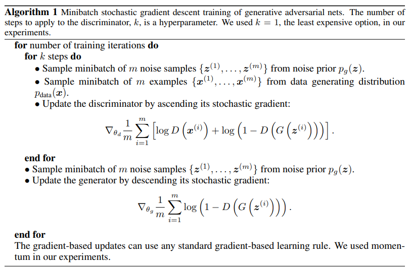
3.2. Algorithm 1
-
Proposition 2
If $G,D$ have enough capacity, and at each step of Algorithm 1, the discriminator is allowed to reach its optimum given G, and $p_g$ is updated to improve the criterion \(min_G max_D V(D,G) = E_{x \sim p_{data}(x)} [log D(x)] + E_{z \sim p_z (z) } [log(1-D(G(z)))]\) then $p_g$ converges to $p_{data}$
-
proof)
consider $V(G,D)= V(p_g ,D)$ as a function of $p_g$ .
Then, by proposition 1, $V(p_g, D)$ is convex around $p_g$
Therefore, if $f(x)$ = $sup_{d \in D} f_d (x)$ is convex in $x$ for every $\alpha$ , then $\partial f_{\beta} (x) \in \partial f$ if $\beta = arg sup_{d \in D} f_{d} (x)$.
This is equivalent to computing a gradient descent update for $p_g$ at the optimal $\mathcal{D}$ given the corresponding $G$. since $sup_D V(p_g, D)$ is unique global optima as proposition 1, therefore with sufficiently small updates of $p_g$, $p_g$ converges to $p_{data}$.
4. Experiment
- on MNIST data, cifar-10, TFD data.
- G used rectifier linear activations, sigmoid mixed. D used maxout activation
- dropout and noise are not allowed in theory. However, noise is used in experiment
-> Generated samples cannot be said better than samples before. However, gan has potential.
5. Pros and Cons
5.1. cons
- no p_{g} explicitly
- $D $, $G$ has to be well-balanced. If one develop too fast, each collapse the other
5.2. pros
- Markov chain is not needed. only back-propagation
- no inference during training
- many models can be applied
- clearer image than markov chains
Leave a comment