[Paper Review] Wasserstein GAN

Date : 2022.11.08 Updated : 2022.11.08

해당 게시글의 참고자료는 다음과 같습니다.

Martin et al. ‘Wasserstein GAN’

Basso, ‘A Hitchhiker’s huide to Wasserstein distance’

전현규님 ‘십분딥러닝_16_WGAN’

임성빈님 ‘Wasserstein GAN 수학 이해하기’

1. Introduction

우리가 어떤 분포를 학습하고자 할 때, 이는 다음 문제를 해결하는 것이다.

\[\begin{align} & ~~~~~\underset{\theta \in \mathbb R ^d}{max} ~\frac{1}{m} \sum _{i=1} ^{m} log P_{\theta} (x^i )\\ & = \underset{\theta \in \mathbb R^d}{min} ~KL(\mathbb P_r \vert \vert \mathbb P_\theta) \end{align}\]
위 문제를 해결하려면 KL Divergence가 계산되어야 하는데, 만약 두 분포의 support 가 겹치지 않는다면 KL Divergence는 발산하게 된다. 즉, 정의되지 않는다.
이를 해결하기 위한 방안 중 하나가 Normal distribution으로부터 noise term을 뽑아내어 추가하는 것인데, 이 경우 support 문제는 해결되나 샘플의 질을 떨어뜨리게 된다.

따라서 $\mathbb{P}_\theta $를 직접 추정하기보다는 $X$를 결정하는 잠재벡터(latent vector) $Z$의 분포를 가정 후 이를 입력으로 받아 Generator를 학습시키는 접근방식이 GAN이다.
그러나 이런 GAN은 여러가지 문제가 발생하는데, 대표적으로 Mode Collapse 문제, Discriminator와 Generator 간 학습의 불균형 등이 있고 이를 해결하고자 Wasserstein Distance를 적용한 게 WGAN 이다.

2. Wassersterin Distance ( = Earth Mover’s Distance)

2.1. Multiple Distances

Notation

$\chi$ : compact metric set

$\Sigma$ : The set of all the Borel subsets of $\chi$

Prob($\chi$) : the space of probability measures defined on $\chi$

위의 notation 하에서, 저자는 다음의 3가지 distance를 먼저 제시한다.

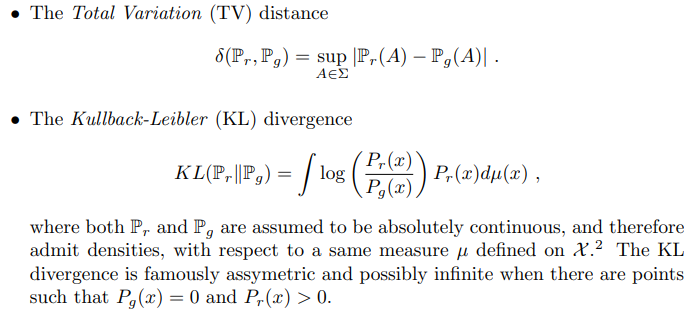
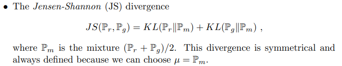
위의 3가지 distance는 기존에 gan관련 논문에서 많이 제시하는 distance들이다.

2.2. EM distances

저자가 논문에서 제시하는 위의 3가지 distance를 대체할 metric은 EM distance이다.

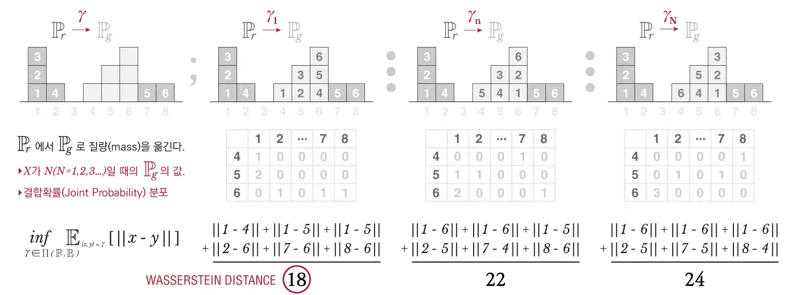
\[\begin{align} &W(\mathbb{P} _r , \mathbb{P}_g) = \underset{\gamma \in \Pi (\mathbb{B}, \mathbb{B})}{inf} \mathbb{E}_{(x,y) \sim \gamma} [\vert \vert x -y \vert \vert] \\& where ~~ \Pi (\mathbb{B}, \mathbb{B})~~is ~~ the ~~set ~~of ~~all~~ joint ~~distributions~~ of ~~\mathbb{P}_r ~~and ~~\mathbb{P}_g \end{align}\]


출처 : (23) 십분딥러닝_16_WGAN (Wasserstein GANs)_2 - YouTube

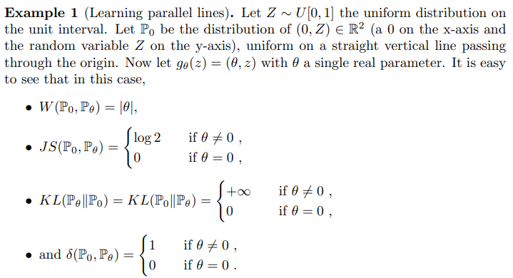
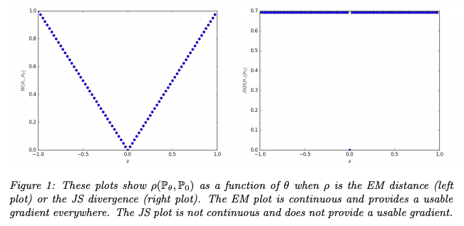
본문에 나와있는 Example 1을 통해 EM distance가 가지는 장점을 알 수 있는데, Parallel Lines 예시를 보면 다른 Metric들은 incontinuous 한 데 반해, EM distance는 continuous 함을 알 수 있다.

이 때 EM distance의 값은 다음과 같이 계산함.

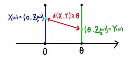
출처 : 임성빈님 ‘Wasserstein GAN 수학 이해하기


출처 : 임성빈님 ‘Wasserstein GAN 수학 이해하기

\[d(X,Y) = (\vert \theta -0 | ^2 + |Z_1 (w) - Z_2 (w) |^2 )^{\frac{1}{2}} \geq \vert \theta \vert\\]

이때, $Z_1 (w ) = Z_2 (w)$이면 최솟값을 달성하므로, EM distance는 $\vert \theta \vert$가 된다.

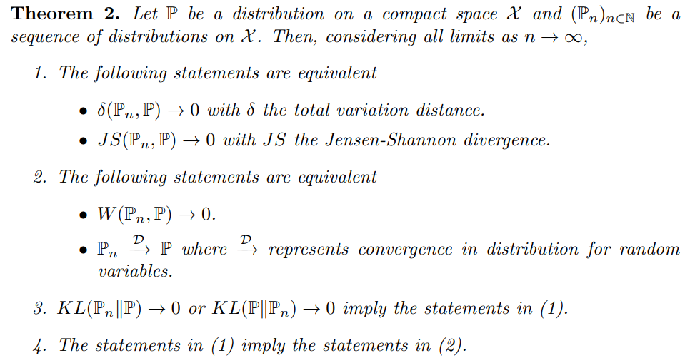
2.3. EM distance 성질

저자에 따르면 EM distance는 KL이나 JS보다 우월한 성질을 지님.
Theorem1에 따르면

Theorem 1.

Let $ \mathbb P_r $ be a fixed distibution over $\chi$ . let $Z$ be a random variable (e.g. Gaussian) over another space $Z$. Let $g$ : $\mathcal{Z} \times \mathbb R^d \rightarrow \chi$ be a function, that will be denoted $g_\theta(z)$ with z the first coordinate and $\theta$ the second. Let $\mathbb P_\theta$ denote the distribution of $g_\theta (Z)$ . Then,

If $g$ is a continuous in $\theta$ , so is $W(\mathbb P_r , \mathbb P_\theta)$

If g is locally Lipschitz and satisfies regularity assumption 1, then $W(\mathbb P_r , \mathbb P_\theta)$ is continuous everywhere, and differentiable almost everywhere.

1-2 are not true for Kullban Leibler and Jensen Shannons

아래의 Corollary를 통해 EM distance의 극소화가 의미 있음을 알 수 있다.

Corollary 1

Let $g_\theta$ be any feedforward neural network parametrized by $\theta$ , and $p(z)$ a prior over $z$ such that $\mathbb E_{z \sim p(z)}[\vert\vert z \vert \vert ] < \infty$ (e.g. Gaussian, uniform, etc.. )

Then assumption 1 is satisfied and $W(\mathbb P_r , \mathbb P_\theta)$ is continuous everywhere and differentiable almost everywhere

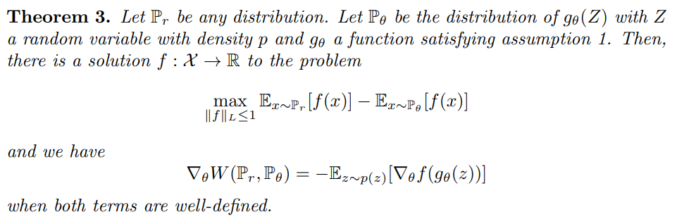
위의 theorem, corollary와 아래의 theorem 2를 생각 시, EM distance가 훈련에 적합한 비용함수라는 것을 알 수 있다.

3.Wasserstein GAN

3.1. Wasserstein GAN approximation

앞서 구한 Wasserstein Distance $W(\mathbb P _r , \mathbb P_g) = \underset{\gamma \in \Pi (\mathbb B, \mathbb B)}{inf} \mathbb E_{(x,y) \sim \gamma} [\vert \vert x -y \vert \vert]$ 는 사실상 계산이 불가능하다. 이를 계산하려면 $x , y$ 의 Joint distribution을 알아야 하는데 $\mathbb P ^r$은 실제 데이터 분포이기 때문.
대신 Kantorovich-Rubinstein Duality Theorem을 통해 근사를 하여서 사용할 수 있다.

for 1 - Lipschitz ($\vert \vert f \vert \vert_L \leq 1$) functions $f ~ : ~ \chi \rightarrow \mathbb R$ ,
\[W(\mathbb P _r , \mathbb P_\theta) = \underset{\vert \vert f \vert \vert \leq 1}{sup} \mathbb E_{x \sim \mathbb P _r} [f(x)] - E_{x \sim p(\theta)} [f(x)]\]

이때, K- Lipschitz로 바꾸면 $K W$의 형태가 되고, 이는 최적화에는 영향을 주지 않으므로 K-Lipschitz를 고려할 수 있다.

for K - Lipschitz ($\vert \vert f \vert \vert_L \leq K$) functions $f ~ : ~ \chi \rightarrow \mathbb R$ ,
\[W(\mathbb P _r , \mathbb P_g) = \underset{w \in \mathcal W}{max} \mathbb E_{x \sim \mathbb P _r} [f_w (x)] - E_{z \sim p(z)} [f_w (g_\theta (z))]\]

Corollary 1에 의해 W 는 almost everywhere differentiable하므로 gradient descent 적용 가능.

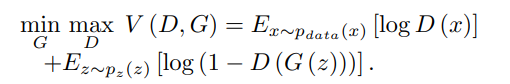
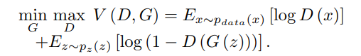
3.2. Objective function

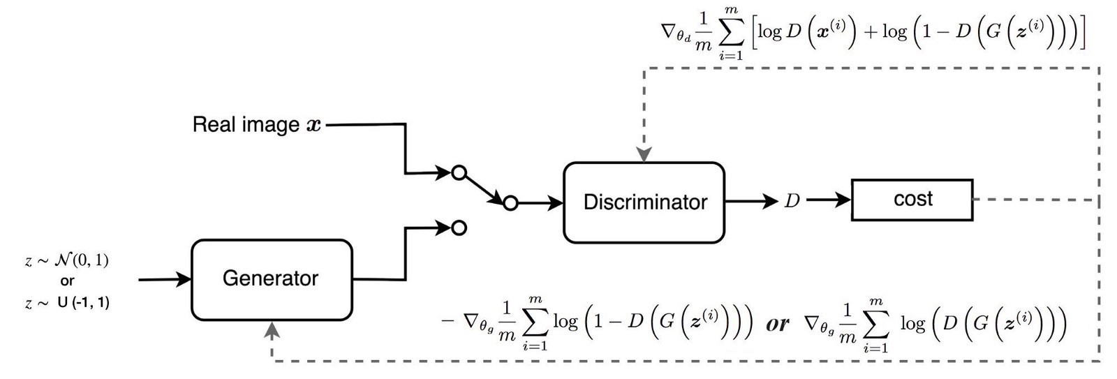
이를 Vanilla GAN과 비교 시 다음과 같다.

Vanilla GAN	Wasserstein GAN

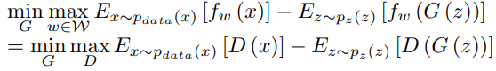차이점은 다음과 같다.

no log in the objective function
D in Vanilla GAN is a binary classifier, while the D in WGAN is a regression task. Therefore, Vanilla GAN includes sigmoid, WGAN do not.
D in WGAN is required to be K-Lipschitz for some K, therefore, WGAN uses weight clipping

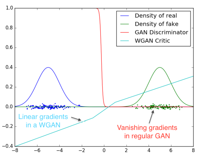
3.3. Smooth Gradient

기존 GAN의 경우 gradient가 폭발하거나, 0이 되거나 하여서 훈련이 잘 되지 않음.
이에 반해, WGAN의 경우 그라디언트가 모든 곳에서 더 매끄러움.

| | | ———————————————————— |

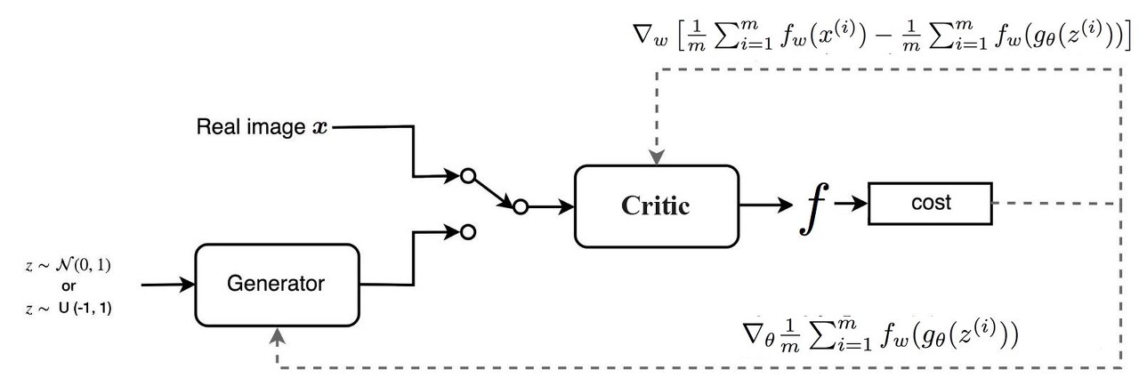
3.4. Structure

WGAN의 경우 critic이 sigmoid function을 가지고 있지 않다는 점을 제외하면 거의 동일.
가장 큰 차이는 cost function에 있음.

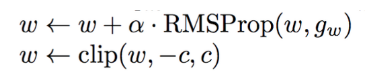
또한, K-Lipschitz 함수여야 하므로, 가중치에 대한 clipping을 적용한다.ㅊ
이때, c 역시 hyperparameter로 작용하며, 적합한 c를 골라야지 훈련이 잘 이루어지게 된다.

(c가 너무 작으면 gradient가 충분히 크지 않아 훈련이 느려지고, c가 너무 크면 기존 vanilla gan에서 발생하는 gradient vanishing 문제가 발생.)

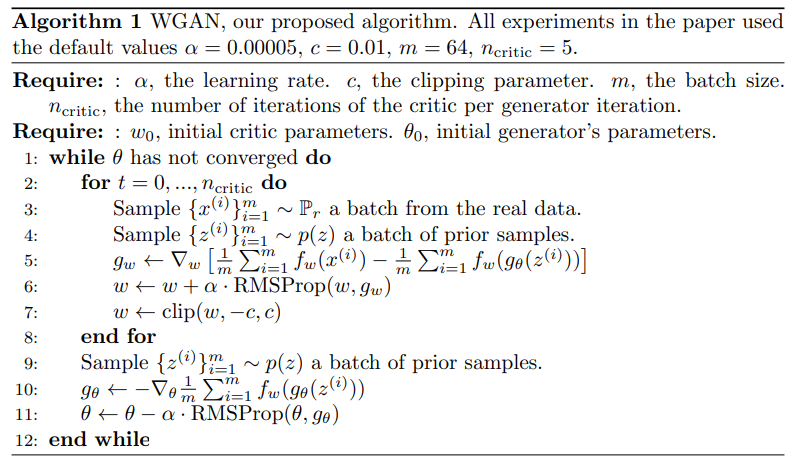
3.5. Pseudo Code

4. Experiment

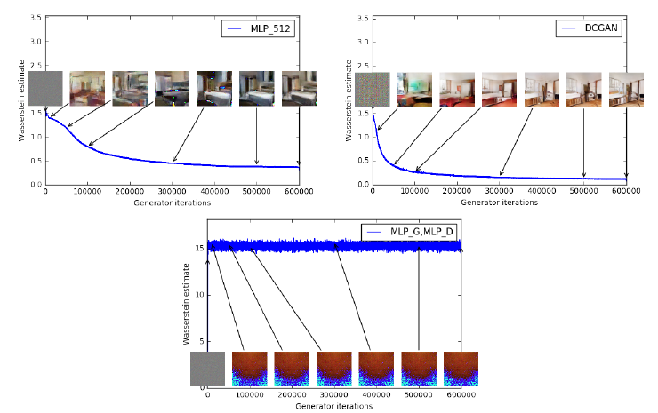
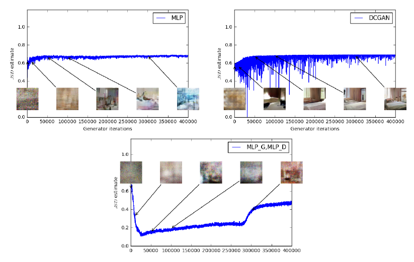
4.1. Cost function and Quality of image

좌측 그래프를 보면, EM Distance와 quality사이의 연관관계가 있음을 확인할 수 있음.
우측 그래프를 보면, JSD와 quality 사이의 연관관계가 없음을 확인할 수 있음.

| | | | ———————————————————— | ———————————————————— |

4.2. Stability

Share on

Twitter Facebook LinkedIn

Insik Cho