[Paper Review] LINE: Large-scale Information Network Embedding

I learned the baseline content about LINE in class Deep learning and Data science at my univ. The slides below came from the class.

The paper is about Network embedding. Especially, this paper deals with the problem of embedding very large information networks into low dimensional vector space. large information networks here mean the big data used in the real world. The paper is

published in 2015, the author said that dealing with really large data was scarce back then.

The paper is cited 4344 times now(2022-05-15). Its core points are 1) considering both local & global networks, and 2) edge-sampling algorithm.

1. Local network(1st order proximity)

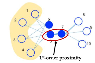
First-order proximity is the direct relationship between two nodes.

For the above example, from the paper, Let’s say if two nodes are connected it has a value of 1 and 0 otherwise (unweighted)

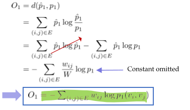
The objective function of 1st order proximity is the distance between empirical probability and the estimated probability

\[O_1 = d(\hat{p_1}, p_1), ~~where ~~\hat{p_1}:~estimated~prob.~~, p_1 : ~empirical~prob.\]

for example, $ \hat{ p_1 } (v_6,v_7) = \frac{1}{5} $, and by optimizing make probability approach to $\frac{1}{5}$

​

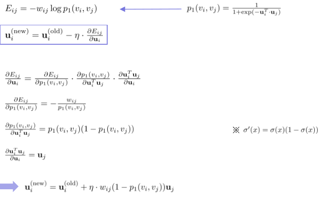
Also, when we call $u_1$ embedding vectors, backpropagation works like

​

2. Global network(2nd order proximity)

second-order proximity is the indirect relationship between two nodes. ‘Indirect’ means that two nodes have similar neighbors.

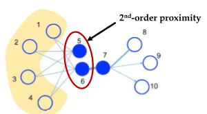
For example, $\hat{p_2} (v_1 \mid v_5) = \frac{1}{4}, ~\hat{p_2} (v_2 mid v_6) = \frac{1}{5} $

Therefore, it tries to approximate the global relationship of vertices.

One can see the difference between first & second proximity with the sentence example ,

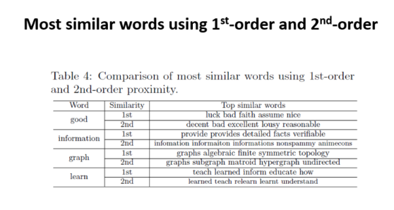
‘information’ has high first-order proximity with providing, details, which are used together with information.

However, high second-order proximity is something like ‘substitutes’, for example, good has bad, excellent as second-order proximity.

3. Negative Sampling

The con of the above algorithm is calculation complexity. from second-order proximity, it requires $O(N^2)$ complexity.

(One can see that denominator is so complex, that it induces high complexity)

Instead, the author suggests using the Negative sampling technique to deal with it.

---

—————————————–Negative Sampling method————————————–

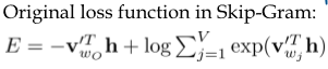
in the original word embedding model, Skip-Gram use the loss above

It came from that

\[p(v_{w_o} \mid w_i) = \frac{exp({v_{w_o }^{'T} \cdot h})}{\sum_j exp({v_{w_i } ^{'T} \cdot h})}\]

and applying -log on it ($- log p$)

New objective ft for negative sampling is

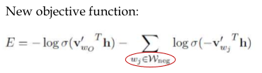
There are two changes.

First, for new one it only implement calculation for selected vertices.

Second, the loss itself is little bit different.

The difference is made from the fact that$\sigma(x) = \frac{1}{1+e ^-x} \sim e^x$

The exact calculation is not going to be specified here.

(check the paper ‘word2vec Explained: Deriving Mikolov et al.’s Negative-Sampling Word-Embedding Method’)

• Noise distribution

we need criteria to vote negative sample. Noise distribution is used for this.

Any distribution can be used, but, the most frequently used one is Unigram distribution.

:The more frequent words are more likely to have higher probabilites.

\[P_n (w_i) = \frac{f_n (w_i)^{3/4}}{\sum\limits _j f_n (w_j)^{3/4}}\]

Here, 3/4 is chosen because it is known to be good empirically, not from analytical analysis.

—————————————–Negative Sampling method————————————–

---

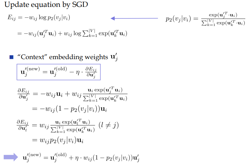
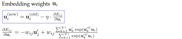
• Negative Sampling for LINE: 2nd proximity.

  The new objective function written above is used for 2nd proximity.

  If we square away the equation, it looks like:

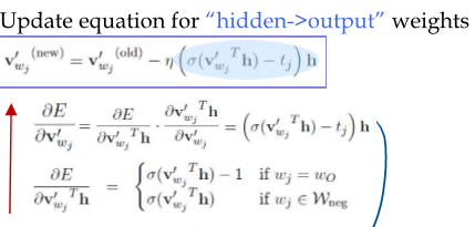
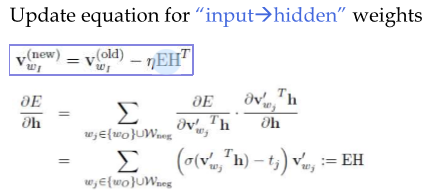
  <Context matrix backpropagation>	<embedding matrix backpropagation>

• Negative sampling for LINE: 1st proximity

It use the objective function : \(log p_1 (v_i,v_j ) = log \sigma (u_j^T u_i) + \sum\limits_{v_n \in neg} log \sigma (- u_n^T u_i)\) It is quite same with above 2nd proximity, just, it does not use context matrix.

Using negative sampling, one can see that the time takes far less for 2nd proximity.

​