[High Dimensional Statistics] Uniform Laws of large numbers

References

• Yonsei univ. STA9104 : Statistical theory for high dimensional and big data
• High-Dimensional Statistics : A Non-Asymptotic Viewpoint, 2017, Martin J. Wainwright

​ Uniform laws have been investigated in part of empirical process theory and have many applications in statics. in contrast to the usual law of large numbers that applies to a fixed sequence of random variables, uniform laws of large numbers provide a guarantee that holds uniformly over collections of random variables. A goal of this post is to introduce tools for studying uniform laws with an emphasis on non-asymptotic results.

1. MotivationPermalink

1.1. Almost sure convergencePermalink

​ Before start of demonstration, I will talk about two probabilistic convergence, Almost sure convergence and Convegence in probability .

1.1.1. Convergence in probabilityPermalink

For $X_n$ and $X$ on ($\mathrm{\Omega },\mathcal{F},\mathbb{P}$), A sequence of random variables converges in probability to a random variable X, denoted by $X_n\stackrel{P}{\to }X$ if

,where $S$ is an underlying sample space.

1.1.2. Almost sure convergencePermalink

For $X_n$ and $X$ on ($\mathrm{\Omega },\mathcal{F},\mathbb{P}$), A sequence of random variables converges almost surely to a random variable X, denoted by $X_n\stackrel{a.s.}{\to }X$ if

,where $S$ is an underlying sample space.

Here, second inequality is true by Borel- Cantelli lemma.

1.1.3. Comparison of conceptsPermalink

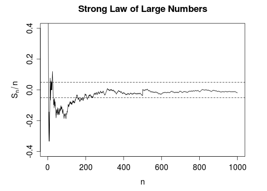
To understand the difference, Law of large number is one example.

I referred random variable - Convergence in probability vs. almost sure convergence - Cross Validated (stackexchange.com) for explanation here.

Weak law of large numbers, which states about convergence in probability of $\overline{X}=\sum _{i=1}^n{X}_i/n$, says that a large proportion of the sample paths will be in the bands on the right-hand side, at time $n$. It just means that the probability that particular curve to be located in curve will approaches to one.

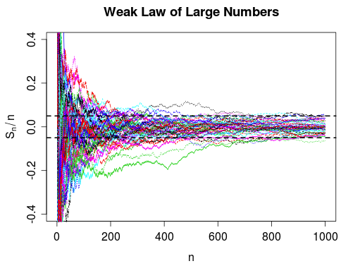
However, in case of strong law of large numbers, a curve surely will be in bands.

The difference also can be seen from other representations of definition.

SLLN

WLLN

, $X_n=\frac{\sum _{i=1}^n{X}_i}{n}$ in case of law of large numbers.

1.2. Cumulative distribution functionsPermalink

Let $X$ be a random variable with its cumulative distribution function, $F(t)=\mathbb{P}(X\le t),\mathrm{\forall }t\in \mathbb{R}$. Then, natural estimate of $F$ is the empirical CDF given by,

${\hat{F}}_n(t)=\frac{1}{n}\sum _{i=1}^n{I}_{(-\mathrm{\infty },t]}(X_i)$ Here, empirical CDF is unbaised estimator for pupulation CDF because

Moreover, uniform convergence of CDF is proved by Glivenko-Cantelli Theorem.

Uniform convergence is important because many estimation problem start from functional of CDF. For example,

• Expectation Functionals

which is estimated by plug-in estimator given by ${\gamma }_g(\widehat{F_n})=\frac{1}{n}\sum _{i=1}^{n}g(X_i)$

• Quantile functionals

which is estimated by plug-in estimator given by $Q_{\alpha }({\hat{F}}_n)=inft\in \mathbb{R}:\widehat{F(t)}\ge \alpha$

Above estimators are justified by continuity of a functional. That is, once we know that $\Vert \widehat{F_n}-F{\Vert }_{\mathrm{\infty }}$ $\to$ 0 in probability, then we also have the result that $|\gamma (\widehat{F_n})-\gamma (F)|\to 0$ for a functional $\gamma$, whenvert $\gamma$ is a continuous with respect to the sup-norm : $\Vert F-G{\Vert }_{\mathrm{\infty }}=su{p}_{t\in \mathbb{R}}|F(t)-G(t)|$

​ continuous with respect to the sup-norm

​ we say that the function $\gamma$ is continuous at $F$ in the sup-norm if, for all $ϵ>0$, there exists a $\delta >0$ such that $||F-G|{|}_{\mathrm{\infty }}\le \delta$ implies that $|\gamma (F)-\gamma (G)|\le ϵ$.

1.3. Uniform laws for more general function classesPermalink

​ Let $\mathcal{F}$ be a class of integrable real-valued functions with domain $\mathcal{X}$ and let ${X_i}_{i=1}^n$ be a collection of i.i.d. samples from some distribution $\mathbb{P}$ over $\mathcal{X}$. consider the random variable

,which measures the absolute deviation between the sample average and the population average, uniformly over the claff $\mathcal{F}$. we say that $\mathcal{F}$ is a Glivenko-Cantelli class for $\mathbb{P}$ if $||{\mathbb{P}}_n-\mathbb{P}|{|}_{\mathcal{F}}$ converges to zero in probability as $n\to \mathrm{\infty }$.

• Empirical CDFs

We could see $\mathcal{F}$ satisfies the definition of Glivenko-Cantelli class by Glivenko-Cantelli Theorem. Therefore, $\mathcal{F}$ is Glivenko-Cantelli class

• Failure of uniform law

Not all classes of functionals are Glivenko-Cantelli. Let $\mathcal{S}$ be the class of all subsets $S$ of $[0,1]$ such that the subset $S$ has a finite number of elements, and consider the function class ${\mathcal{F}}_S=I_S(\cdot ):S\in \mathcal{S}$ of indicator functions of such sets. Suppose that samples are drawn from continuous distributions over $[0,1]$ such that $\mathbb{P}(S)=0$ for any $S\in \mathcal{S}$ . on the other hand, for any positive interger $n\in \mathbb{N}$, the discrete set $S_n=X_1,\cdots ,X_n$ belongs to $\mathcal{S}$, and moreover, by definition of the empirical distribution, we have

Therefore, we conclude that

, and thereby ${\mathcal{F}}_{\mathcal{S}}$ is not a Glivenko-Cantelli class for continuous distributions.

1.4. Empirical risk minimizationPermalink

• Suppose that samples are drawn i.i.d. according to a distribution ${\mathbb{P}}_{{\theta }^{\star }}$ for som fixed but unknown ${\theta }^{\star }\in \mathrm{\Omega }$.
• A standard approach to estimating ${\theta }^{\ast }$ is based on minimizing a cost function ${\mathcal{L}}_{\theta }(X)$ that measures the fit between a parameter $\theta \in \mathrm{\Omega }$ and the sample $X\in \mathcal{X}$.
• We then obtain some estimate $\hat{\theta }$ that minimizes the empirical risk defined as

​ One specific example is Maximum Likelihood Estimator.

• In contrast, the population risk is defined as

​ where expectation is taken over a samples $X\sim {\mathbb{P}}_{{\theta }^{\star }}$. The statistical question of interest is how to bound the $excessrisk$:

​ Which is risk from estimor of empirical risk minimization and true unknown estimator is how small compared to pupulation risk.

​ For simplicity, assume that there exists some ${\theta }_0\in \mathrm{\Omega }$ such that $R({\theta }_0,{\theta }^{\star })=\underset{\theta \in \mathrm{\Omega }}{inf}R(\theta ,{\theta }^{\star })$

With the notation , the exess risk can be decomposed as

By the definition of $\hat{\theta }$, $T_2<0$. For the $T_1$,

, uniform law of large numbers over the cost function $\mathcal{F}(\mathrm{\Omega })=x\to {\mathcal{L}}_{\theta }(x),\theta \in {\mathrm{\Omega }}_0$ is required. With this notation,

Also, for the $T_3$ , is dominated by this quantity,

It is also dominated by above quantity,

It states that the central challenge in analyzing estimators based on empirical risk minimization is to establish a uniform law of large numbers for the loss class $\mathcal{F}(\mathrm{\Omega })$.

2. A uniform law via Rademacher complexityPermalink

2.1. Definition of Rademacher complexityPermalink

• Empiricial Rademacher complexity of the function class $\mathcal{F}$

For any fixed collection $x_1^n=(x_1,\cdots ,x_n)$, consider the subset of ${\mathbb{R}}^n$ given by

The empirical Rademacher complexity is given by

, where ${ϵ}_1,\cdots ,{ϵ}_n$ are $i.i.d.$ Rademacher random variables.

• Rademacher complecity of the function class $\mathcal{F}$

​ By taking expectation on empirical rademacher complexity,

​ By the form of formula, note that the Rademacher complexity is the maximum correlation between the vector $(f(x_1),f(x_2),\cdots f(x_n))$ and the noise vector (${ϵ}_1,\cdots ,{ϵ}_n$). Also, if a function class is extremply large, then we can always find a function that has a high correlation with a randomly drawn noise vector. Conversely, if function size is too small, correlation will be small.

​ In this sense,the Rademacher complexity measures the size of a function class and it plays a key role in establishing uniform convergence resuts.

2.2. Glivenko-Cantelli propetyPermalink

• $Define)$ a function class $\mathcal{F}$ IS $b$-uniformly bounded if $||f|{|}_{\mathrm{\infty }}\le b$ for all $f\in \mathcal{F}$.

• Theorem (Glivenko-Cantelli property) For any $b$-uniformly bounded class of function class $\mathcal{F}$ , any positive integer $n\ge 1$ and any scale $\delta \ge 0$, we have

​ with $\mathbb{P}$ -probability at least $1-\exp (-\frac{n{\delta }^2}{2b^2})$. Consequently, as long as ${\mathcal{R}}_n(\mathcal{F})=o(1),$ we have $||{\mathbb{P}}_n-\mathbb{P}|{|}_{\mathcal{F}}\stackrel{a.s.}{\to }0$.

proof)

• Borel-Cantelli lemma

Let $ϵ>0$ and define

Borel-Cantelli lemma says that if $\sum _{i=1}^{\mathrm{\infty }}\mathbb{P}(A_n(ϵ))<\mathrm{\infty },then{X}_n\stackrel{a.s.}{\to }X$

For above case,

Therefore, since $\sum _{n=1}^{\mathrm{\infty }}\exp (-\frac{n{\delta }^2}{2b^2})<\mathrm{\infty }$, the Borel-Cantelli lemma guarantees $\lVert \mathbb{P} n -\mathbb{P} \rVert{\mathcal{F} } \overset{a.s.}{\rightarrow} 0$ from the statement. Accordingly, the remainder of the argument is devoted to proving the inequality,

which will lead to uniform convergence of CDF .

• Step 1) concentration around mean

Let’s say that $\Vert {\mathbb{P}}_n-\mathbb{P}{\Vert }_{\mathcal{F}}:=G(X_1,\cdots ,X_n)$. Then, to show the concentration around the mean, I will show the bounded difference condition of $G$ with $max{L}_i\le \frac{2b}{n}$.

$\begin{array}{rl}& |\frac{1}{n}\sum _{i=1}^n(G(X_1,\cdots ,X_n)-\mathbb{E}[G(X_1,\cdots ,X_n)])|-\underset{G\in \mathcal{F}}{sup}|\frac{1}{n}\sum _{i=1}^n(G(Y_1,\cdots ,Y_n)-\mathbb{E}[G(Y_1,\cdots ,Y_n)])|\\ & \le |\frac{1}{n}\sum _{i=1}^n(G(X_1,\cdots ,X_n)-\mathbb{E}[G(X_1,\cdots ,X_n)])|-|\frac{1}{n}\sum _{i=1}^n(G(Y_1,\cdots ,Y_n)-\mathbb{E}[G(Y_1,\cdots ,Y_n)])|\\ & \le \frac{1}{n}|\sum _{i=1}^n(G(X_1,\cdots ,X_n)-\mathbb{E}[G(X_1,\cdots ,X_n)])-\sum _{i=1}^n(G(Y_1,\cdots ,Y_n)-\mathbb{E}[G(Y_1,\cdots ,Y_n)])|\\ & \le \frac{2b}{n}⟵b-uniformlybounded\\ & ⟶suponeachside\\ & G(X_1,\cdots ,X_n)-G(Y_1,\cdots ,Y_n)\le \frac{2b}{n}\end{array}$

Then, by McDiard’s theorem ,

with probability at least $1-exp(-\frac{n{t}^2}{2b^2})$.

• Step 2) Upper bound on the mean

Combining results, one can get given inequality.

3. Upper bounds on the Rademacher complexityPermalink

3.1. Polynomical discriminationPermalink

Definition ( Polynomial Discrimination)

A class $\mathcal{F}$ of functions with domain $\mathcal{X}$ has polynomial discrimination of order $\nu \ge 1$ if, for each positive integer $n$ and collection $x_1^n=\{x_1,\cdots ,x_n\}$, the set

has cardinality upper bound as

The significance of this property is that it provides with a straightforward approach to controlling the empirical Rademacher complexity

3.2. Bound on the empirical Rademacher complexityPermalink

Suppose that $\mathcal{F}$ has polynomial discrimination of order $\nu$. Then, for all positive integers $n$ and any collection of points $x_1^n=(x_1,\cdots ,x_{)},$

, where $D(x_1^n)=\underset{f\in \mathcal{F}}{sup}\sqrt{\frac{1}{n}\sum _{i=1}^n{f}^2(x_i)}$ is the ${\mathcal{l}}_2$ - radius of the set $\mathcal{F}(x_1^n)/\sqrt{n}$.

proof)

For any fixed vector $a=(a_1,\cdots ,a_n)\in {\mathbb{R}}^n$, the random variable $\frac{1}{n}\sum _{i=1}^n{ϵ}_i{a}_i$ is sub-Gaussian with variance proxy ${\sigma }^2=\frac{1}{n^2}\sum _{i=1}^n{a}_i^2$ . Since $\mathcal{F}$ has polynomial discrimination of order $\nu$, there are at most $(n+1{)}^{\nu }$ vectors of the form $(f(x_1),\cdots ,f(x_n))$, and each such vector has $l_2$- norm bounded by

Therfore, the empirical Rademamcher complexity is upper bounded by the expected supremum of $(n+1{)}^{\nu }$ Rademacher variables, each with variance proxy at most $D^2(x_1^n)/n$. Applying maximal inequality of sub-Gaussian, it yields that

• one of maximal inequality used here

Let $X_1,\cdots ,$ be zero-mean sub-Gaussian random variables with proxy ${\sigma }^2$

Then, $\mathbb{E}[\underset{1\le i\le n}{max}|X_i|]\le \sigma \sqrt{2log(2n)}$

3.3. Glivenko-Cantelli theroemPermalink

Corlloary (Glivenko- Cantelli)

Let $F(t)=\mathbb{P}(X\le t)$ be the CDF of a random variable $X$, and let ${\hat{F}}_n$ be the empirical CDF based on $n$ i.i.d. sample $X_i\sim \mathbb{P}$. Then, for all $\delta >0$ and $n\ge 1$,

with probability at least $1-\exp (-\frac{n{\delta }^2}{2b^2})$. Therefor, $\Vert F-{\hat{F}}_n{\Vert }_{\mathrm{\infty }}\stackrel{a.s.}{\to }0$

proof )

Because for a givne sample $x_1^n=(x_1,\cdots ,x_n)$ and function class $\mathcal{F}=\{I_{(-\mathrm{\infty },t]}(\cdot ):t\in \mathbb{R}\}$, consider the set $\mathcal{F}(x_1^n)=\{f(x_1),\cdots ,f(x_n):f\in \mathcal{F}\}$. Because it only divides real line into $n+1$ parts, cardinality is $n+1$, which means that polynomial discrimination of order 1. Then, by the results above, given inequalities works.

3.4. Vapnik-Chervonenkis dimensionPermalink

Above, we see that Polinomical discrimination is useful to find the upper bound. One of way to verify that a given function class has polynomial discrimination is via the thoery of VC dimension. Consider a function class $\mathcal{F}$ where each function $f$ is binary-valued, {0,1} for simplicity. Then the set $\mathcal{F}(x_1^n)$ has at most $2^n$ elements. (Of course, because each element has 2 possibilities).

Definition (VC dimension) Given a class $\mathcal{F}$ of binary-valued functions, we say that the set $x_1^n=(x_1,\cdots ,x_n)$ is shattered by $\mathcal{F}$ if card($\mathcal{F}(x_1^n))=2^n$. The VC dimension $\gamma (F)$ is the $largest$ interger $n$ of which there is some collection $x_1^n=(x_1,\cdots ,x_n)$ of $n$ points that is shatter by $\mathcal{F}$.

• Example : Two-sided Intervals in $\mathbb{R}$

Consider the collection of all two-sided intervals over the real line – namely ${\mathcal{S}}_{\mathcal{both}}=(b,a]:a,b\in suchthatb<a$. The class ${\mathcal{S}}_{both}$ can shatter any two distinct points. However, given three distinct points $x_1<x_2<x_3$, it is not possible to pick out the subset {$x_1,x_3$}, showing that the VC dimension $\nu ({\mathcal{S}}_{both})=2$.

• Sauer’s Lemma

Consider a set class $\mathcal{F}$ with the VC dimension $\gamma (\mathcal{F})<\mathrm{\infty }$. Then, for any $n>\gamma (\mathcal{F})$, we have that

$card(\mathcal{F}(x_1^n))\le (n+1{)}^{\gamma (\mathcal{F})}$

3.5. Multivariate version of Glivenko-CantelliPermalink

Theorem

Let $X_1,\cdots ,X_n$ be $i.i.d.$ obesrvations frnom a distribution $P$ on ${\mathbb{R}}^d$ . let $F$ denot the multivariate cumulative distribution function of $P$, that is

where for vectores $\mathbf{x}\mathbf{=}\mathbf{(}{\mathbf{x}}_{\mathbf{1}}\mathbf{,}\cdots \mathbf{,}{\mathbf{x}}_{\mathbf{d}}\mathbf{)}$ and $\mathbf{y}\mathbf{=}\mathbf{(}{\mathbf{y}}_{\mathbf{1}}\mathbf{,}\cdots \mathbf{,}{\mathbf{y}}_{\mathbf{d}}\mathbf{)}$ in ${\mathbb{R}}^d$ , $\mathbf{x}\le \mathbf{y}$ means that $x_j\le y_u$ for all $j=1,\cdots ,d$. Let ${\hat{F}}_n$ denote the empirical CDF of $P$, i.e.

Then,

, with probability at least $1-exp(-\frac{n{\delta }^2}{2})$.

proof)

At first, class of indicator functions characterized by the class of sets $\mathcal{A}=(-\mathrm{\infty },x_1](-\mathrm{\infty },x_2]\times (-\mathrm{\infty },x_d],(x_1,\cdots ,x_d\in {\mathbb{R}}^d)$ has VC dimension $d$.

because $\mathcal{A}$ has VC-dimension $d$, apllying sauer’s lemma, for fixed $x_1^n$ , we haver

, which means that $\mathcal{F}$ has polynomical discrimination of order $d$.

Because class $\mathcal{F}$ is 1-uniformly bounded (Because it is CDF), implement Glivenko-Cantelli property, for any positive interger $n\ge 1$ and any scale $\delta \ge 0$, we have

with probability at least $1-exp(-\frac{n{\delta }^2}{2})$, which is,