[Linear Model] One-way ANOVA

1. ANOVA table

1. 1. Problem set up

A one-way ANOVA can be written as

\[Y_{ij} = \mu + \alpha_i + \epsilon_{ij}\]

where $E(\epsilon_{ij}) =0 , \,\,var(\epsilon_{ij}) = \sigma^2, $ and $cov(\epsilon_{ij}, \epsilon_{i’j’} ) =0$. Also, assume $\epsilon_{ij} \sim N(0,\sigma^2)$ for hypothesis testing.

If we write the above problem as

\[Y = X \beta + \epsilon\]

, $X = [j_n ,X_1 , \cdots, X_t]$, where $X_k = (x_{11}, … , x_{1n_1}, \cdots, x_{t1}, \cdots, x_{tn_t})’, $ $x_{ij} = I(i=k)$

Thus, $X_k$ has exactly $n_k$ ones and $n-n_k$ zeros.

1.2. Decomposition of SST

​ The usual orthogonal breakdown for a one-way ANOVA is to isolate the effect of the global mean($\mu$), and then the effect of fitting the groups($\alpha_i$) after fitting the mean. The sum of squares for treatment($SS_{trt}$) is just what is left after removing the sum of squares for $\mu (SS_{gm})$ from the sum of squares for the model. In other words, $SS_{trt}$ is the sum of squares for testing the reduced model against the full model.

​ We can easily check that orthogonal projection operator for $SS_{gm}$ is $M_\mu = \frac{1}{n} J_n$ and for whole variables is $M = blkdiag(\frac{1}{n_1} J_{n_1}, \cdots , \frac{1}{n_t} J_{n_t} )$. The orthogonal projection operator for $SS_{trt}$ is then,

\[M_\alpha = M- M_\mu\]

​ Therefore, decomposition of $Y’Y $ is,

\[\underset{SST}{Y'Y} = Y' (I-M)Y + Y'MY = \underset{SSE}{Y'(I-M)Y} + \underset{SS_{gm}}{Y'M_\mu Y} + \underset{SS_{trt}}{Y'M_\alpha Y}\]

1.3. ANOVA table with matrix form

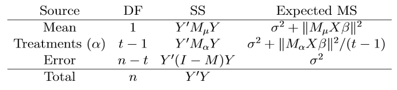
Here, the next theorem is used:

\[E(Y'AY) = tr(A \Sigma) + \mu' A \mu\]

​ An F-test for no treatment effect, which is $H_0 : \alpha_1 = \cdots = \alpha_t$ can be constructed by ANOVA table above. It is easy to verify that,

\[\frac{Y'M_\alpha Y/ (t-1)}{Y'(I-M)Y / (n-t)} \sim F(t-1, n-t, \gamma)\]

,where $\gamma = \frac{\vert \vert M_\alpha X \beta \vert \vert^2}{2 \sigma^2} $, which is 0 under $H_0$

1.4. ANOVA table with scalar form

Some notes about One way ANOVA :

2. Contrasts

2.1. Side conditions

‘Side conditions’ are extra conditions to get ‘estimators’ of non estimble quantities, for example $\alpha_i$ in 1-way anova.

Example: $\sum_{i=1}^t n_i \alpha_i =0$

With the condition, $\mu = \frac{1}{n }\sum_{i=1}^t n_i (\mu + \alpha_i)$. Therefore, $\mu$ can be estimated by the estimators of $\mu + \alpha_i$, which are estimable.

\[\hat{\mu} = \frac{1}{n} \sum n_i \bar{Y_{i.}} = \frac{1}{n} \sum_{i=1}^t \sum_{j=1}^{n_i} Y_{ij} = \bar{Y_{..}}\]